Generative Art
Definitions are tricky.
What is generative art? It is "generative" in that the artist uses some kind of system or rules or process to create it. These rules often involve a random component, although they don't have to.
As for the "art" part, Galanter03 speaks of "artistic complexity" as a way of framing the space. He argues that the place where "art" lives in this context is where there is complexity, understood as peaking between pure randomness and pure order. He applies some lessons from complexity theory to understanding and defining generative art. A completely predictable arrangement is boring; a purely random arrangement is baffling. Therefore: boring. The aesthetic sweet spot falls where there is some amount of predictability, but also some surprise.

Complete regularity is boring

Artistic complexity is somewhere in the middle
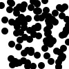
Complete random noise is boring
Artistic complexity by this account forms a U-shaped curve, low where there is complete regularity, peaking in the middle, and falling again as we descend into randomness. Generative art can be formed by sprinkling just the right amount of randomness onto regular patterns, or by using a sufficiently complicated system, even if it has no random element. Great complexity can also emerge from simple iterated systems.
Frequently generative art is created using computer algorithms to produce digital works or to drive plotters. There are also generative artists who create hand-drawn works, where the random element comes from rolling dice or flipping coins. Examples of non-random generative art includes renderings of fractals or the complexity of Islamic tiling.
Whether the complexity comes from the complexity of the underlying system, from the emergent complexity of iterated simple rules, or from randomness, it is still up to the artist to make aesthetic selections. Fractal art derives from specific deterministic functions: the art lies in making decisions about selecting which parts of the function to show and how to render it. Simple Lindenmeyer systems (discussed more in section “String Manipulation”) are completely non-random, just the repeated application of simple string rewrite rules. Yet they can still produce some pleasing results: here the aesthetic determination is in which system to implement and how to map it to a visual rendering. For randomized art, selecting and perhaps mashing up the best experiments is part of the artistry.
The generative art discussed here uses algorithms with a random component to create visual digital works.
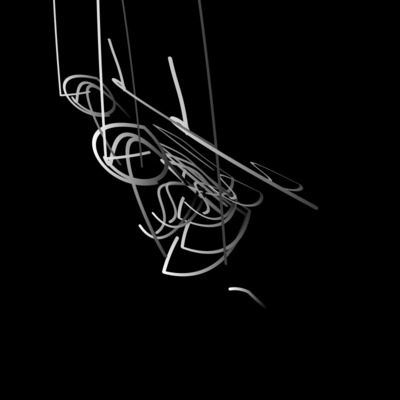
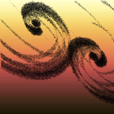
Generative artwork, iterated random swooshes
Creating such an artwork involves embarking on an iterative process of experimentation: initiation, generation, selection, adjustment, and consolidation. An algorithm is created, a set of works are created with that algorithm, aesthetic judgement is applied to pick which experiments to preserve and how to tweak the algorithm, and then we try again, possibly followed by some manual post-editing or mash-up on selected works. In the consolidation phase, components of works are encapsulated to form the basis of new derived works. Artistic complexity is thus built up over time through a hierarchy of named components of increasing intrinsic complexity.
|
Initiation |
The creation of an algorithm, with some random component. The algorithm may be inspired by some natural phenomenon, some specific aesthetic target, a regular pattern, or some other work. |
|
Generation |
A series of experiments are run using the algorithm. Given the random component, some of these may work out well, and some not so well. Some algorithms produce more consistently appealing results, some not so much. The latter require more experiments. |
|
Selection |
Here is where artistic judgement is applied. Some outputs may be taken as is, or taken as a more promising direction and used to determine how to tweak the algorithm or adjust weights to bias the random selections in a particular direction. Since this is a programming task, debugging happens at this stage, too, although unlike the debugging of many programming tasks, sometimes the bug produces an interesting effect, that might become the deliberate outcome in the next project. Serendipity! |
|
Adjustment |
The algorithm is tweaked, parameters and weights are shifted, stylings and renderings are messed with, before the process heads back to the next iteration cycle of generation/selection/adjustment. It is possible that manual adjustment may be applied to selected works. |
|
Consolidation |
It is common to construct variations on a common theme by taking components of one work and using them in some way in another. Encapsulating components for reuse supports this activity. |
What then is needed to produce generative art?
|
Rendering engine |
Again, the end goal is to produce a visual artifact. Therefore, some means of displaying the works is required. This could be using the browser to natively render some digital artifact, or feeding a set of instructions to a mechanical plotter. |
|
Programming substrate |
Work begins by authoring a generating program. Such a program executes in a particular environment: a particular programming language with a particular set of ancillary libraries. There are as many possibilities here as there are computer languages: JavaScript and Python are popular, but Flash, Java, special purpose tools and scripting languages are also used. |
|
Randomizers |
Aesthetically interesting complexity may come from a complex algorithm, or a set of rules that interact in complex ways, but at base there is generally some kind of random component to the algorithms. The algorithms will benefit from being able to produce random numbers in accordance with various probability distributions. The programming substrate often provides some kind of randomizer (or pseudo-randomizer); more complex distributions may need to be built on top of that. |
|
Operations |
The end goal of this effort is to produce visual artifacts: images laid out in two dimensional space. It is useful to have supporting mathematical and geometric operations to allow the calculation of the placement of visual elements within that space. Certain kinds of algorithms benefit from capable string operations. |
|
Components |
Reusable components allow for the construction of more interesting works based on high-level concepts. Encapsulating interesting pieces of one work can allow the generation of variations based on a common aesthetic element. |
|
Aesthetic judgement |
Aesthetic judgement ultimately comes from the artist. One might, however, apply machine learning techniques or genetic algorithms to mechanically converge on more fruitful parts of the parameter space of a particular algorithm, or for post-processing. |
|
Tracking |
It may not be immediately obvious, but for experimentation to progress, one must keep track of which experiments succeeded, and which failed; which produced more pleasing outcomes, and which did not. This can be approached as a scientific endeavour, where the lab notebook is king. |
My Approach
My target artifact is SVG, rendered directly in the browser or via ImageMagick. The programming substrate is the XML stack, especially XQuery and XSLT. For randomizers I built an XQuery library on top of a single built-in function. Many of the operations were available in the programming substrate, either as standard built-in functions and operators, or as extensions available in the particular engine I use. I developed XQuery libraries and XSLT stylesheets to support more idiosyncratic components. Keeping track of experiments has evolved from note taking and source control to a more systematic framework.
I am not claiming this is the best way to make generative art or the only way. There are many paths, with different pros and cons.
|
Rendering engine |
SVG rendered by browser or ImageMagick |
|
Programming substrate |
XQuery and XSLT with library functions |
|
Randomizers |
Library built on top of a built-in function that generates random numbers |
|
Operations |
Standard XQuery and XSLT functions and operators, platform-specific built-ins, and library functions |
|
Components |
XQuery and XSLT libraries with an evolving set of design elements and components |
|
Aesthetic judgement |
Me, looking and editing |
|
Tracking |
A framework of parameter tracking and timestamping, combined with source control and a lab notebook |
Rendering engine
SVG is rendered in the browser or via ImageMagick, usually directly in the editor (Emacs). Being able to render in the editor, which can also toggle the display to the generated source, while having the source algorithm in a companion buffer is very handy. Minor tweaks can be tested quickly by making small edits before adjusting the algorithms or the rendering parameters.
The other thing rendering to SVG gives you is the ability to look at the SVG as XML and glean something meaningful from it. In the browser the view source functionality provides this, and in Emacs it is a keystroke away. True, XML is not always the most readable textual format, and SVG is not always the most readable XML format. But consider JPEG. View source would be hopeless.
Especially when you start to veer into areas of SVG you aren't very familiar with, view source can be crucial. What is art, but the exploration of the unfamiliar? The broken rendering or blank screen is an all-too common result. Are the points out of the range of the canvas? Is there a missing or misspelled class definition? Did the code get embedded instead of the results of executing the code? View source can answer these questions.

A likely output of any new art project
Programming substrate
SVG is an XML dialect. I use XQuery and XSLT to generate it. Pilot experiments with any particular algorithm often start with direct generation of SVG out of XQuery, followed by a shift to generating XML in a domain-specific language which is converted to SVG with XSLT. XQuery is more convenient for implementing complex algorithms and libraries for randomizers, geometric operations, or special systems and components. XSLT is great for translating domain-specific XML and adding colours and stylistic effects. The domain-specific language elements sometimes start off as somewhat generic and low-level, with the more interesting pieces being peeled off into higher-level domain-specific elements later. As I have developed more components, the initial algorithms have become more high-level. New projects can leverage and combine complex components, creating more complex components in turn.
In this way, I can increase artistic complexity without increasing the mental and programming burden.
The Power of Small Domain-Specific Languages
The problem with SVG is that while, yes, it is XML, key parts are designed for compactness,
not for manipulation. For example, consider the snippet of SVG in Figure 1. The paths consist of a coded series of operators (M, A, and C) and control points. The transforms consist of a series of operators concatenated
together. While it is easy enough to generate strings in output, manipulating a series
of geometric paths (for example, to prune crossing paths) requires that we operate
at a higher level.
Figure 1: SVG snippet
...
  <g transform="translate(-56 -50) scale(0.875 0.875) skewX(10) skewY(9)">
    <g transform="scale(1 1) skewX(2.489)">
      <path d="M 340 543
               A 540 487 -17.161 0 0 291 629 312 621 -4.358 0 0 512 465
               C 389 396 467 376 343 367 420 452 544 542 355 380"
            class="Swoosh" style="stroke-width:7"/>
    </g>
  </g>
  <g transform="translate(-62 -50) scale(0.75 0.75) skewX(19) skewY(17)">
    <g transform="scale(1 1) skewX(2.489)">
      <path d="M 340 543
               A 540 487 -17.161 0 0 291 629 312 621 -4.358 0 0 512 465
               C 389 396 467 376 343 367 420 452 544 542 355 380"
            class="Swoosh" style="stroke-width:7"/>
    </g>
  </g>
  <g transform="translate(-68 -50) scale(0.625 0.625) skewX(25) skewY(25)">
    <g transform="scale(1 1) skewX(2.489)">
      <path d="M 340 543
               A 540 487 -17.161 0 0 291 629 312 621 -4.358 0 0 512 465
               C 389 396 467 376 343 367 420 452 544 542 355 380"
            class="Swoosh" style="stroke-width:7"/>
    </g>
  </g>
...
Compact path and transform strings in a snippet of SVG.
Having made the decision to create the algorithms using higher level constructs, there is actually a considerable advantage to emitting those higher level constructs as well. This allows me to abstract some of the messy geometric details, and even postpone some of the rendering choices. Now I can test variations in the fundamental algorithms separately from variations in rendering.
It is the classic separation of content and form in a new guise: the separation of algorithmic aesthetic choices from stylistic aesthetic choices.
Consider the scrap of domain-specific XML in Figure 2. The algorithm and its randomizers make decisions about the number and lengths of threads and drops. In this case, initial experiments focused on the overall shape of the threads. I shifted the thread length algorithm from the same normal distribution for each thread to one where the mean was the length of the preceding thread. A fixed default rendering was applied in this phase of the process to enable me to make such aesthetic judgements.
Figure 2: Generated source
<art:canvas width="720" height="720" ...>
  <art:thread x="6">
    <art:drop y="0" length="20"/>
    <art:drop y="25" length="13"/>
    <art:drop y="43" length="15"/>
    <art:drop y="63" length="15"/>
  </art:thread>
  <art:thread x="24">
    <art:drop y="0" length="26"/>
    <art:drop y="31" length="9"/>
    <art:drop y="45" length="20"/>
    <art:drop y="70" length="12"/>
  </art:thread>
  <art:thread x="34">
    <art:drop y="0" length="15"/>
    <art:drop y="20" length="29"/>
    <art:drop y="54" length="26"/>
  </art:thread>
   ...
</art:canvas>
Example of generated domain-specific output. Elements are partially shared between
projects (e.g. art:canvas) and partially specific to a particular project (e.g. art:drop).
With the raw output in hand, the next phase of experimentation can render the same basic form in many different ways. This allows for a somewhat "scientific" approach to the experimentation: limiting what I vary at any given moment to see what works best overall.
Figure 3: Using small domain-specific language to vary effects

Default rendering parameters

Small adjustment (max-stroke-width=8)

More radical shape adjustment (drop-shape=chevron)
Various renderings of same set of randomized drop threads
Note that we are not necessarily talking about small stylistic variations here. The entire shape can be rendered in entirely different ways.
It can be tricky to decide where to draw that line.
Consider the iterated random swooshes in section “Generative Art”. The concept of an "echo", where a design element is repeated several times but offset,
skewed, and shrunk slightly with each repetition, plays heavily there. It comes up
in a lot of my other works as well. It would be tempting to create an echo element in the DSL which just has a count of how many echoes to make. However, using
the same degree of offset, skew, and shrinkage in each echo is boring (too orderly),
so echoes are created with slight random variations in these values. But if I want
to keep randomization out of rendering, I have a problem, and either echo never makes it to the DSL, or it becomes much more complex with specific information
about how the shape is modified in each repetition, blunting the utility of an echo
element in the DSL in the first place. An intermediate position is to make a library
function for creating echoes of a base shape.
What is manifest in the DSL versus what is introduced in the stylesheet versus what is a library function is a fluid and evolving boundary. The result has been elements at various levels from quite abstract all the way down to SVG pass-through. A particular project or set of related projects often move from less abstract to more abstract as work proceeds.
Stylesheet Framework
Transforming the domain specific language is the job of a set of stylesheets, which
are organized with a set of defined parameters and customization layers, similar to
the setup with the DocBook stylesheets (see DocBook). There is a main shared stylesheet (render.xsl) which includes a stylesheet that defines various parameters (param.xsl). The entry-point stylesheet for any particular project imports the main shared stylesheet
and overrides various parameters and templates as required. The entry-point stylesheet
will also define parameters and templates for elements that are specific to that project.
Figure 4 shows a project-specific entry-point stylesheet. It functions as a customization
layer on top of the imported render.xsl. In addition to overriding default values for several standard parameters (stroke-class and max-stroke-width), and specifying values for the hooks for project-specific information (project-style-defs and project-styles), it defines several project-specific parameters (drop-shape et al). The project-specific element art:drop has a template that defines how it should be rendered to SVG.
Figure 4: Transforming to SVG
<!-- Entrypoint stylesheet: render-thread.xsl -->
<xsl:stylesheet xmlns:xsl="http://www.w3.org/1999/XSL/Transform" ...>

  <xsl:import href="render.xsl"/>

  <!-- Overrides for default parameters -->
  <xsl:param name="stroke-class">BlueSwoosh</xsl:param>
  <xsl:param name="max-stroke-width">4</xsl:param>

  <xsl:param name="project-style-defs">
    <svg:linearGradient id="BlueGradient"
         gradientUnits="userSpaceOnUse"
         x1="0" x2="0" y1="0" y2="50"
    >
      <svg:stop offset="0%" stop-color="#FFFFEE" />
      <svg:stop offset="100%" stop-color="#0000E0" />
    </svg:linearGradient>
  </xsl:param>

  <xsl:param name="project-styles">
    .BlueSwoosh {
      fill:none;
      stroke:url(#BlueGradient);
      stroke-linecap:<xsl:value-of select="$stroke-cap"/>;
      stroke-linejoin:<xsl:value-of select="$stroke-join"/>
    }
  </xsl:param>

  <!-- Project-specific parameters -->
  <xsl:param name="drop-shape">line</xsl:param>
  <xsl:param name="drop-fill">none</xsl:param>
  <xsl:param name="drop-opacity">1</xsl:param>
  <xsl:param name="gap">5</xsl:param>

...
  <!-- Project-specific templates -->
  <xsl:template match="art:drop">
    <svg:g transform="translate(0,{@y + $gap*count(preceding-sibling::art:drop)})">
      <svg:g class="{$stroke-class}"
             stroke-width="{max((1,$max-stroke-width - (@y idiv 100)))}">
        <xsl:choose>
...
          <xsl:when test="$drop-shape='chevron'">
            <svg:path d="m 0 {$gap} L -5 {@length} m 0 {$gap} L 5 {@length}"/>
          </xsl:when>
          <xsl:when test="$drop-shape='circle'">
            <svg:circle cx="0" cy="{$gap + (@length idiv 2)}" r="{@length idiv 4}"
                        fill="{$drop-fill}" fill-opacity="{$drop-opacity}"/>
          </xsl:when>
          <xsl:otherwise>
            <svg:path d="m 0 {$gap} L 0 {@length}"/>
          </xsl:otherwise>
        </xsl:choose>
      </svg:g>
    </svg:g>
  </xsl:template>
</xsl:stylesheet>
Stylesheet to generate SVG from domain-specific sources. Note that "styling" may mean rendering completely different kinds of shapes.
Figure 5 shows the base shared stylesheet. The main base stylesheet provides templates for
shared elements (e.g. art:canvas). A separate included stylesheet (param.xsl) defines various parameters. The stylesheet uses several modes to provide projects
the means to put information into the appropriate part of the SVG result: as metadata,
as definitions to be referenced, or as body content to be rendered.
Figure 5: Transforming to SVG: Base stylesheet
<!-- Base stylesheet: render.xsl -->
<xsl:stylesheet xmlns:xsl="http://www.w3.org/1999/XSL/Transform" ...>

  <xsl:include href="param.xsl"/>

  ...

  <xsl:template match="/">
    <xsl:apply-templates select="*"/>
  </xsl:template>

  <xsl:template match="art:canvas">
    <svg:svg version="1.1"
      width="{@width}px" height="{@height}px"
      viewBox="0 0 {@width} {@height}"
    >
      <xsl:apply-templates select="." mode="metadata"/>
      <svg:defs>
        <xsl:apply-templates select="." mode="defs"/>
      </svg:defs>
      <svg:style type="text/css">
        <xsl:apply-templates select="." mode="styles"/>
      </svg:style>
      <svg:g>
        <xsl:apply-templates select="." mode="body"/>
      </svg:g>
    </svg:svg>
  </xsl:template>

  <!-- Embed metadata -->
  <xsl:template match="art:canvas" mode="metadata">
    <xsl:apply-templates select="art:metadata"/>
    <xsl:if test="empty(art:metadata)">
      <art:metadata style="display:none">
        <xsl:call-template name="dump-parameters"/>
      </art:metadata>
    </xsl:if>
  </xsl:template>

  <!-- SVG defs -->
  <xsl:template match="art:canvas" mode="defs">
    <xsl:copy-of select="$global-style-defs"/>
    <xsl:copy-of select="$project-style-defs"/>
    <xsl:apply-templates select="* except art:metadata" mode="defs"/>
  </xsl:template>

  <!-- CSS styles -->
  <xsl:template match="art:canvas" mode="styles">
    <xsl:copy-of select="$global-styles"/>
    <xsl:copy-of select="$project-styles"/>
    <xsl:apply-templates select="* except art:metadata" mode="styles"/>
  </xsl:template>

  <!-- Main body:
       Do children in body mode for any background elements
       In default mode to the rest
    -->
  <xsl:template match="art:canvas" mode="body">
    <xsl:variable name="fill">...</xsl:variable>
    <xsl:variable name="opacity">...</xsl:variable>
    <xsl:variable name="filter">...</xsl:variable>
    <svg:rect x="0" y="0" width="{@width}" height="{@height}">
      <xsl:if test="$fill ne ''">
        <xsl:attribute name="fill">
          <xsl:value-of select="$fill"/>
        </xsl:attribute>
      </xsl:if>
      <xsl:if test="$opacity ne ''">
        <xsl:attribute name="opacity">
          <xsl:value-of select="$opacity"/>
        </xsl:attribute>
      </xsl:if>
      <xsl:if test="$filter ne ''">
        <xsl:attribute name="filter">
          <xsl:value-of select="$filter"/>
        </xsl:attribute>
      </xsl:if>
    </svg:rect>
    <xsl:apply-templates select="* except art:metadata" mode="body"/>
    <xsl:apply-templates select="* except art:metadata"/>
  </xsl:template>

  ...
  <!-- vertical arrangement of objects, e.g. drops -->
  <xsl:template match="art:thread">
    <svg:g transform="translate({@x},0)">
      <xsl:apply-templates/>
    </svg:g>
  </xsl:template>

  <!-- horizontal line of objects, e.g. glyphs -->
  <xsl:template match="art:line">
    <svg:g transform="translate(0,{@y})">
      <xsl:apply-templates/>
    </svg:g>
  </xsl:template>
...
</xsl:stylesheet>
Base stylesheet shared by different projects.
Finally, as components evolve, some of the project-specific templates and parameters migrate into component stylesheets, which can then be used by later projects.
Randomizers
The underlying engine (in this case MarkLogic) provides a single uniform random number generator. In this case it generates integers
between 0 and some specified upper bound. It was therefore necessary to create a library
of functions to provide other distributions such a normal, skewed normal, Zipf, Markov
chains, multimodal, and so on. Implementing some of these depends on the availability
of various mathematical operations. With adjustments, similar generators can be implemented
on top of any such random or pseudo-random number generator[1] such as the XQuery 3.1 function random-number-generator.
Implementing these distributions was not all that challenging. Algorithms are widely
described. Here, for example, is an implementation of the normal distribution. The
function rand:uniform() produces a double value between its two parameters (inclusive), a slight extension
over the platform's randomizer.
Figure 6: Implementing normal distribution
(:
 : normal()
 : Return random normally distributed data.
 :
 : $mean: Mean of range of values
 : $std: Standard deviation of range of values
 :)
declare function rand:normal(
  $mean as xs:double,
  $std as xs:double
) as xs:double
{
  $mean + rand:gauss() * $std
};

(:
 : gauss()
 : Return random normally distributed data between 0 and 1
 : A service function used by normal()
 :)
declare %private function rand:gauss() as xs:double
{
  let $u as xs:double := 2 * rand:uniform(0,1) - 1
  let $v as xs:double := 2 * rand:uniform(0,1) - 1
  let $r := $u * $u + $v * $v
  return (
    if ($r = 0 or $r >= 1) then rand:gauss()
    else (
      let $c as xs:double := math:sqrt(-2 * math:log($r) div $r)
      return $u * $c
    )
  )
};
Implementation of a function to produce normally distributed random numbers with a particular mean and standard deviation.
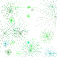
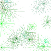
Why have multiple distributions? Many generative artists seem content to stick with a default uniform distribution. This surprises me, given that the distribution can have a profound effect on the final outcome and a uniform distribution does not always give the best result.
Figure 7: Different size distributions
Uniform distribution
Normal distribution
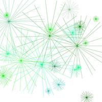
Bimodal distribution
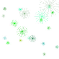
Zipf distribution
A set of random starbursts created using the same distributions for everything except sizes. Size ranges are the same in each case.
A few important considerations come into play in implementing randomizers and the APIs for using them: performance, uniformity, and sequences. Given the general utility of a randomizer library, there is some value in limiting the platform dependence here too, even though I am less concerned about that for more idiosyncratic levels of the stack.
Randomizers will be called in the tightest inner loop of the algorithm. The more complex (i.e. interesting) the artwork, the more they will be called. Performance is important. Maybe not "running the weather prediction on the supercomputer" important, but not trivial either. Given that these are randomizers for art, not for cryptographically secured banking, accuracy of the algorithm in producing a particular distribution is of secondary consideration. The algorithm shown above for generating random numbers in a normal distribution is an approximation, although a decent one (Boiroju12).
One way the performance requirement manifests in the APIs is in the passing of (precalculated) cumulative probability sums. There are functions that can pre-compute these for a particular distribution, and binary search is used to make selections at a particular probability level very efficiently.
It turns out the underlying platform also embeds the CNTK machine learning library, which includes functions to generate values from some of the distributions of interest. Why not just use them? Surely that would provide the best performance? In fact, no. It turns out that the mechanics of preparing data in and out of them it not entirely trivial and has a substantial overhead: it runs almost twice as slowly as the XQuery implementation even when generating large numbers of values in one go and almost four times as slowly when generating one value at a time. CNTK is designed for executing large complicated models on a large amount of data, not calling one-off functions. So here the demands of performance also accord with the sentiment to avoid egregious platform dependence at this level.
Taken in the context of a cycle of experimentation and tweaking, it is useful to have a single API entry point that can generate different distributions of numbers based on a bundle of parameters. This turns the selection of a distribution into a declarative act. One can tweak the parameter bundle without having to change the code at all. Here I use a map to hold the parameters.
For Markov chains, the previous value generated is required to produce the next value. Even for non-Markov chains, frequently one wants to base the specifics of the current value on the previous value in some way. As we saw in the example in Figure 2, one thread's length correlated with the value of the previous one, by using the length of the previous thread as the mean for the new random length.
A couple of more minor considerations: random numbers are used in a variety of contexts. Sometimes it is important that the final result be an integer, or confined to a particular range or, for the sake of readability and the size of the output files, restricted to two decimal points. The randomizer API provides hooks for this as well.
Figure 8: Generic Randomizer API
(:
 : randomize()
 : Main entry point for randomizers.
 :
 : $n: How many values to return
 : $last: Previous value (needed for markov, also available to key callback)
 : $algorithm: The algorithm to use, a map with various parameter keys
 :   distribution: Distribution to use, one of "constant", "uniform", "normal",
 :     "skewed", "bernoulli", "flip", "zipf", "markov", "sums", "multimodal"
 :   min: minimum value (optional)
 :   max: maximum value (optional)
 :   pre-multiplier: multiplier before min/max (optional)
 :   post-multiplier: multiplier after min/max (optional)
 :   cast: cast type (optional)
 :   mean: mean of distribution (normal, skewed) (default=0)
 :   std: standard deviation of distribution (normal, skewed) (default=mean)
 :   skew: skew of distribution (skewed) (default=0)
 :   p: probability (bernoulli, flip) (default=50)
 :   sums: cumulative probability sums (zipf, markov, sums)
 :   alpha: alpha parameter (zipf) (needed if no sums) (default=0)
 :   limit: number of sums (zipf) (needed if no sums) (default=1000)
 :   start: index of starting symbol (markov) (default=uniform[1,dim])
 :   dim: size of each dimension of Markov matrix (markov)
 :   matrix: raw Markov matrix (used if sums not provided; not recommended)
 :   distribution: sequence of distributions to combine (multimodal)
 :   truncation: how to keep value in [min,max] range (all but constant/uniform)
 :     ceiling => ceiling/floor to min/max
 :     drop => toss out (so may return < $N)
 :     resample (default) => resample until an in-bound value is found or
 :       resample limit is reached (then use ceiling)
 :)
rand:randomize(
  $n as xs:integer,
  $last as item()?,
  $algorithm as map(xs:string,item()*)
) as item()*
The generic randomizer interface generates a number of random numbers according to the given algorithm parameters.
A non-obvious aspect of the rand:randomizer API is that each numerical parameter in the map can be replaced by a callback function
that takes the current algorithm map and the previous value generated. This allows
me to generate sequences of values that depend on each other without having to modify
the map.
The full randomizer library includes a number of useful functions besides the main entry point: functions to scramble a set of values, select a value based on a particular randomized index, and print out a nice histogram of values to see what a particular algorithm's distribution looks like.
Operations
XPath (and thus XQuery) provides many useful operations across a variety of data types.
Mathematics
All algorithms rely on basic arithmetic operations: addition, subtraction, division, multiplication. Modulus and calculations of minimums and maximums come into play sometimes as well.
The randomizer library depends on a number of standard mathematical XPath functions,
as we saw in Figure 6, such as math:pi, math:sqrt, math:pow. Various standard shapes depend on these as well, such as the shape function that
generates the starbursts we saw in Figure 7.
Geometry
Trigonometric functions are crucial. Creating the branching tree of Figure 10, for example, requires being able to compute a destination point giving a starting point, an angle, and a stroke length, which means using sines and cosines. Standard XPath functions provide the basics here.
It is useful, however, to have more. The underlying engine provides a comprehensive set of extensions for geospatial data types and operations such as region intersection or distance between points. These can all be applied in a flat coordinate system. That is: they function as useful (Euclidean) geometric functions. Despite a general inclination to encapsulate platform dependencies, the geospatial data types (especially the point data type) were too compelling to avoid or hide.
A library is layered on top of the base geospatial functions to provide some basic utility and convenience functions, however. It also makes things easier in an SVG environment. For example, points in SVG space are integers in x-y space over a visible canvas, not floating point numbers in latitude-longitude space, so the library defines x and y coordinate accessors and functions to snap points to the grid, constrain them to the canvas, and scale back and forth between the unit square and the canvas.
Key geometric operations here are implemented using the operations provided by the underlying platform, but they could be implemented using basic mathematical and trigonometric functions, if necessary. Other engines may implement their own geometric capabilities, perhaps following the EXPath geospatial API.
Figure 9: Using geometric functions
...
let $hull := geom:convex-hull($shape)
let $center := geom:centroid($hull)
let $distance := 1.2 * geom:distance-from-center($hull, "max")
let $angle := rand:randomize($BEARING)
let $new-start-point := geom:point-at($center, $angle, $distance)
...
A snippet of code that uses geometric calculations to create a starting point separated somewhat from a current polygonal shape.
String Manipulation
Basic string operations come into play for creating the SVG data: concatenation and
normalization. There is heavy use of the standard XPath functions string-join, concat, and normalize-string.
Lindenmeyer systems are systems of string rewriting rules. Stochastic Lindenmeyer
systems add a probability to certain rules, creating alternative rewrite pathways.
Such systems can be a very powerful means of creating naturalistic and complex forms.
The rewrite rules run over several generations to create a coded string. For example,
the strings generated for Figure 10 look like ...[[X]-X]+F[-FX]+X]+F+[[X]-X]-F[... That string then needs to be parsed and interpreted and converted into something
to be rendered. Here F means draw a line in current direction, + means turn to the right, and so on. In my framework translation means generating
some domain specific XML.
Figure 10: L-system tree
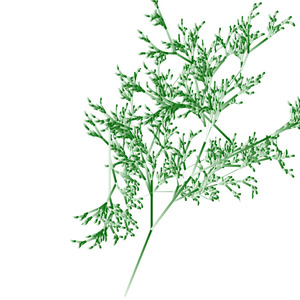
Tree generated with stochastic Lindenmeyer system
Depending on the complexity of the system and the mapping, more or less powerful string
matching and manipulation functions are required. Basics such as string-to-codepoints, substring-before, and substring-after, as well tokenize and the power-tool analyze-string get a lot of use.
Higher-order Functions
It might not seem obvious at first, but fold-left sees a lot of action. Wherever we need to compute a value that depends on the previously
computed value it pops up: Markov sequences, probability distribution sums, Lindenmeyer
systems, and as a basis of many algorithms (such as the one behind the examples in
Figure 3). Figure 11 shows how fold-left is used in computing Zipf cumulative probability sums.
Figure 11: Zipf probability sums
declare function rand:zipf-sums(
  $α as xs:double,
  $n as xs:integer
) as xs:double*
{
   let $c :=
     fold-left(
       function($z,$i) {
         $z + 1 div (math:pow(xs:double($i), $α))
       },
       0,
       1 to $n
     )
   let $c := 1 div $c
   return
     fold-left(
       function($z,$i) {
         $z,
         $z[last()] + $c div math:pow(xs:double($i), $α)
       },
       0,
       1 to $n
     )[position() gt 1] (: skip initial 0 :)
};
Using fold-left to compute Zipf probability distribution sums.
Higher-order functions come into play with the generic randomizer function. It provides for function callback hooks for each parameter, which depends on the ability to have function values in the algorithm map and the ability to invoke such functions. The execution framework also relies on function callbacks to generate metadata and content.
Maps
Maps are used to hold randomizer specifications, as we have already seen. The execution framework uses maps to hold algorithm and rendering parameter values and pass these bundles of values in a consistent way. XML could be used for these purposes, but it ends up being messier especially with respect to function callbacks. Maps also come into play a great deal for various data structures because implementations optimize the "update" operations on them so that high-count iterative algorithms can perform reasonably.
Components
Components arise in an ad hoc fashion based on refactoring of previous works at both the algorithmic and the rendering levels: base shapes and arrangements, algorithms for manipulating base shapes, rendering widgets, and so on.
Shapes, Paths, Systems, and Components
Libraries containing methods for creating various interesting shapes and paths evolve as building blocks for future work. For example, the path library has methods to construct a set of points around a circle, in a spiral, along a meandering line, in an array of lines, and so on. There are optional randomizer parameters to jitter the placement. Other libraries have methods for creating various interesting shapes. Base shapes can be modified in various ways: another library has methods for this. Laying out modified base shapes along different modified base paths creates distinct variations on a base work.
More specific and complex kinds of components get their own libraries: particular systems for generating asemic glyphs, for example, or particularly interesting Lindenmeyer systems and their interpretations that produce interesting branchings. Standard methods can execute stochastic and non-stochastic rewrite systems of various kinds.
Figure 12: Spiral murmurations
declare function this:content()
{
  let $density := $ACTIVE-PARAMETERS=>map:get("density")
  let $generations := $ACTIVE-PARAMETERS=>map:get("generations")
  let $scale := $ACTIVE-PARAMETERS=>map:get("scale")
  let $spiral-in := path:golden-spiral($density,$generations,$scale)
  let $width := rand:randomize($WIDTH)
  let $spiral-out := geom:translate(reverse($spiral-in),$width,$width)
  let $base-shape := ($spiral-in, $spiral-out, $spiral-in[1]) (: close loop :)
  for $i in 1 to rand:randomize($SEEDS)
  let $shape :=
    if (rand:randomize($REFLECT))
    then
      geom:reflect($base-shape,
        geom:point(0,0),
        geom:point($CANVAS=>map:get("width"), $CANVAS=>map:get("height")))
    else $base-shape
  let $shape := geom:rotate($shape, rand:randomize($ANGLE))
  let $point := path:random-point($CANVAS)
  for $i in 1 to rand:randomize($ECHOES)
  let $mutant := geom:scale(geom:shear($shape, $i, $i), 1 - ($i - 1) div 10)
  let $shift := geom:translate($point,($i - 1)*2,($i - 1)*2)
  return (
    <art:spiral x="{geom:x($shift)}" y="{geom:x($shift)}">{
      art:points($mutant)
    }</art:spiral>
  )
};
Using a standard Fibonacci spiral path, with reflection and iteration
This is an area of active and continual development.
Experimental Framework
The general process for running tests is the same for each algorithm, to the point where I have abstracted a lot of mechanics into a standard template and set of support functions. A set of external variables define whether I am performing a new experiment or rendering a previous one, how many trials to generate, what customization layer to use, what changes to the default parameters to apply, and so on. A standard experiment driver is invoked, passing in the appropriate variables and two function arguments that create the core content and the metadata block, respectively. Outputs are tagged with a date and time stamp, a project label, and a variant label for alternative renderings.
A project generator then boils down to a set of standardized variables, a couple of functions that will be used as callbacks by the driver, and an invocation of the driver itself. Where the algorithm is reusing component shapes, paths, or systems from a previous project, it can become quite simple.
In order to allow maximum flexibility in running tweaks without having to edit the specific XQuery algorithm, both algorithm parameters and rendering parameters can be passed into generator as external variables. These are merged with the default set of parameters, overriding existing values with the same key, and preserving any non-shared keys, with the merged sets being passed on to the driver.
Colours, Gradients, and Visual Effects
It is always easier to track and manage parameterized and named design elements.
SVG provides for 150 named colours. That's nice, but I want more, including all the
Emacs colour names. I created scripts to merge the base SVG colour names with the
colours in the Emacs rgb.txt file to create an XSLT stylesheet with a colour table and a lookup function for each
colour name. As a small bit of overkill, there is a named parameter for each colour
name whose value is the RGB value of that colour or SVG native colour name. Other
rendering stylesheets can reference colours via parameter names directly or via the
lookup function. For example, the parameter named RoyalBlue3 has the value #3A5FCD. Passing a value of RoyalBlue3 as the background-fill value will invoke the lookup function to set the background to that particular shade
of blue.
Automatic generation of simple gradients and styles by name is also provided. The
stylesheet parameter palettes drives this. It is a space delimited set of names. A palette named simple-X generates a CSS class of the same name that produces strokes in the colour X. A palette
named white-to-X generates a definition for a simple gradient from white to the colour X and a style
to go with it. A palette named black-to-X generates a definition for a simple gradient from black to the colour X and a style
to go with that. Any of the colour names can be used. So black-to-RoyalBlue3 creates a simple gradient definition from #000000 (black) to #3A5FCD (RoyalBlue3) and a CSS style of the same name. Elements in the DSL conventionally
take a class attribute to attach such styling to the rendering of the component.
I make great use of the gradients created by Crameri. His purpose was to make gradients for scientific use that are perceptually ordered
and uniform, while maintaining these properties in the face of colour-vision deficiency
or even in black-and-white print. The perceptual uniformity and ordering make them
pleasing in artistic works also. A couple dozen gradients are provided in a variety
of formats, including SVG. I created stylesheets for each gradient which wrap the
SVG gradient definition in an XSLT parameter with the same name. Each of the Scientific
Colour Map gradients is quite large, with 512 gradient stops, so including them all
in every generated SVG would be unwieldy. When the palettes parameter includes the given name, the corresponding definition is added to the SVG
along with a corresponding CSS class, but not otherwise.
Several variations of all gradients are possible using naming conventions to reverse
the sense of the gradient, to put the gradient against the y axis instead of the x
axis, or to sweep both at the same time, or to create a circular gradient instead
of a linear one. These simple variations are sufficient to capture most of the use
cases, but it is always possible to use the project-style-defs stylesheet parameter, SVG passthrough, or the template override for the defs mode as an escape hatch. There is also a convention for naming each colour stop in
a gradient.
Figure 13: Parameterized gradient inclusion
<!-- gradients.xsl -->
  <!-- Each of these stylesheets contains one gradient definition: -->
...
  <xsl:include href="COLOURS/tokyo.xsl"/>
  <xsl:include href="COLOURS/turku.xsl"/>
  <xsl:include href="COLOURS/vik.xsl"/>
...
  <!-- Look up or generate SVG gradient definition -->
  <xsl:function name="art:gradient-definition">
    <xsl:param name="name"/>
    <xsl:choose>
      <!-- Named gradients -->
      <xsl:when test="$name='acton'"><xsl:copy-of select="$acton"/></xsl:when>
      <xsl:when test="$name='bamako'"><xsl:copy-of select="$bamako"/></xsl:when>
      ...
      <!-- Convention for simple gradients -->
      <xsl:when test="starts-with($name,'black-to-')">
        <xsl:variable name="stop-colour">
          <xsl:value-of
            select="art:colour(substring-after($name,'black-to-'))"/>
        </xsl:variable>
        <svg:linearGradient id="{$name}"
          gradientUnits="objectBoundingBox" spreadMethod="pad"
          x1="0%" x2="100%" y1="0%" y2="0%"
        >
          <svg:stop offset="0%" stop-color="#000000"/>
          <svg:stop offset="100%" stop-color="{$stop-colour}"/>
        </svg:linearGradient>
      </xsl:when>
      <xsl:otherwise/>
    </xsl:choose>
  </xsl:function>
  ...
  <!-- Modify linear gradient (across x) to inverted gradient across x -->
  <xsl:template name="reverse">
    <xsl:param name="def"/>
    <svg:linearGradient id="{$def/*/@id}-reverse"
      gradientUnits="objectBoundingBox" spreadMethod="pad"
      x1="100%" x2="0%" y1="0%" y2="0%"
    >
      <xsl:copy-of select="$def/*/*"/>
    </svg:linearGradient>
  </xsl:template>
  ...
  <!-- Modifying linear gradient to an inverted circular gradient -->
  <xsl:template name="inflow">
    <xsl:param name="def"/>
    <svg:radialGradient id="{$def/*/@id}-inflow"
      gradientUnits="objectBoundingBox" spreadMethod="pad"
      cx="50%" cy="50%" r="50%"
    >
      <xsl:variable name="offsets" as="xs:string*">
        <xsl:sequence as="xs:string*" select="$def/*/*/@offset"/>
      </xsl:variable>
      <xsl:variable name="colors" as="xs:string*">
        <xsl:sequence as="xs:string*" select="reverse($def/*/*/@stop-color)"/>
      </xsl:variable>
      <xsl:variable name="opacities" as="xs:string*">
        <xsl:sequence as="xs:string*" select="reverse($def/*/*/@stop-opacity)"/>
      </xsl:variable>
      <xsl:for-each select="1 to count($offsets)">
        <xsl:variable name="i" as="xs:integer" select="."/>
        <svg:stop
          offset="{$offsets[$i]}"
          stop-color="{$colors[$i]}"
          stop-opacity="{$opacities[$i]}"/>
      </xsl:for-each>
    </svg:radialGradient>
  </xsl:template>

<!-- param.xsl -->
...
  <!-- Pulled into the defs part of the SVG file -->
  <xsl:param name="global-style-defs">
    <xsl:variable name="gradients"
      select="distinct-values(
        tokenize(concat($palettes,' ',$stroke-class),' ')[. ne ''])"
    />
    <xsl:for-each select="$gradients">
      <xsl:variable name="name" select="."/>
      <xsl:variable name="root"
        select="replace($name,
          '(-reverse|-flip|-invert|-full|-anti|-outflow|-inflow)','')"
      />
      <xsl:choose>
        <!-- Gradient across decreasing x -->
        <xsl:when test="ends-with($name,'-reverse')">
          <xsl:call-template name="reverse">
            <xsl:with-param name="def">
              <xsl:copy-of select="art:gradient-definition($root)"/>
            </xsl:with-param>
          </xsl:call-template>
        </xsl:when>
        <!-- Gradient across increasing y -->
        <xsl:when test="ends-with($name,'-flip')">
          <xsl:call-template name="flip">
            <xsl:with-param name="def">
              <xsl:copy-of select="art:gradient-definition($root)"/>
            </xsl:with-param>
          </xsl:call-template>
        </xsl:when>
        ...
        <xsl:otherwise>
          <xsl:copy-of select="art:gradient-definition($root)"/>
        </xsl:otherwise>
      </xsl:choose>
    </xsl:for-each>
    ...
  </xsl:param>

  <!-- Pulled into the CSS style definitions part of SVG output: -->
  <xsl:param name="global-styles">
    ...
    <xsl:variable name="gradients"
      select="distinct-values(
        (tokenize($palettes,' '),$stroke-class)[. ne ''])"/>
    <xsl:for-each select="$gradients">
      <xsl:variable name="name" select="."/>
      <xsl:choose>
        <xsl:when test="starts-with($name,'basic-')">
          .<xsl:value-of select="$name"/> {
          stroke:<xsl:value-of
            select="art:fill(substring-after($name,'basic-'))"/>;
          stroke-linecap:<xsl:value-of select="$stroke-cap"/>;
          stroke-linejoin:<xsl:value-of select="$stroke-join"/>;
          stroke-opacity:<xsl:value-of select="$stroke-opacity"/>;
          <xsl:if test="$stroke-fill ne ''">fill:<xsl:value-of
            select="art:fill($stroke-fill)"/></xsl:if>
          }
        </xsl:when>
        ...
        <xsl:otherwise>
          .<xsl:value-of select="$name"/> {
          stroke:url(#<xsl:value-of select="$name"/>);
          stroke-linecap:<xsl:value-of select="$stroke-cap"/>;
          stroke-linejoin:<xsl:value-of select="$stroke-join"/>;
          stroke-opacity:<xsl:value-of select="$stroke-opacity"/>;
          <xsl:if test="$stroke-fill ne ''">fill:<xsl:value-of
            select="art:fill($stroke-fill)"/></xsl:if>
          }
        </xsl:otherwise>
      </xsl:choose>
    </xsl:for-each>
  </xsl:param>
Some of the tooling for gradient and colour style generation
A similar, but less systematic scheme, is available for defined filters to provide
various visual effects. In this case it is the stylesheet parameter effects that drives the inclusion of the various filter definitions and styles. Here the
set of available effects is a growing ad hoc collection of interesting effects using
SVG filters, such as drop shadows, glows, 3D lighting effects, splotchification, and
so on.
Figure 14: Incised characters
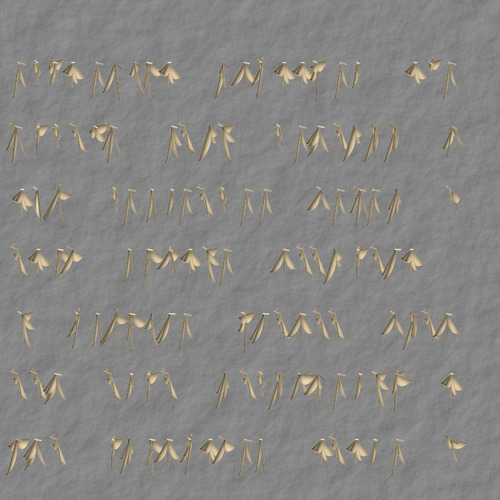
Using colour-parameterized stone effect for background, incised effect on glyph strokes
Improving the tooling, the set of available effects, and standardizing on more of the key parameters is ongoing work. The tooling for filters is somewhat weak at the moment.
Aesthetic judgement
Judgement is applied by selecting from a set of generated works. Following the split between the generation of the domain-specific language outputs and the generation of the SVG, there are two distinct phases of judgement. In the first, basic default styling is used over variations in the algorithm. In the second, variations of styling are used over fixed DSL outputs. In each phase, the best set of those variations is selected to proceed with. Sometimes, a very fast edit/render cycle in the editor on the final SVG is applied to inform decisions about how to adjust the stylesheets (or the algorithms) so that a more desirable outcome can be generated without interventions.
Tracking
The process of creating generative art is one of repeated cycles of tinkering. Experiment, tweak, review, experiment, tweak, review. Sometimes you want to take a piece from some other project and apply it to a new project. Sometimes it is the "failures" from a previous project that you want to pick up and run with in a new context. What were those parameters that worked? What was that algorithmic tweak? It is easy to lose track. An average project generates hundreds of candidate works every day.
Whenever software is being written, a good source control system and methodology shouldn't be far behind. Here I stood up a quick local instance of Subversion (SVN). For a single-user codebase this is less about branching and merging, and more about checkpointing. Substantive versions of new projects get committed as work proceeds. This fails to capture a lot of the tinkering, however. More is needed.
I took three other steps to keep track:
-
Lab notebook
-
Timestamping outputs
-
Automatic metadata embedding
The "lab notebook" is a plain text file kept ready to hand in a buffer at all times. Here I keep notes about the experiments as they happen, interspersed with date and time markers. This gets committed at the end of each day and reviewed each morning. It is also a place for jotting down ideas about things to try. Keeping a running log of my work has been a practice since graduate school, and I highly recommend it as both a memory aid and as a way of seeing your own progress. There are limitations: sometimes the notes in the notebook end up being too terse. Being too verbose creates a burden and barrier to actually keeping it up. Post-editing at the end of the day can help here.
Figure 15: Lab notebook
* 0322
8:50 start crack algorithm; artlib dump-parameters
pm too hard to translate, try lsystem
* 0323
9:30 fix bug in lsystem render -- looks like vines, but I like it
9:48 x2/y2 = abs(...) mod width/height
10:14 reset M for x2/y2 shifted to get rid of straight lines
* 0324
Adding sand
colours.xsl
A few (overly terse) lines from the lab notebook.
In a mad cycle of tinkering, it can be hard to keep up even with the lab notebook, and not every parameter tweak seems worthy of another commit. It can also be hard to associate a particular outcome with a particular version of the software and the parameters. Having a framework that keeps track of some of this automatically is helpful.
Embedded Metadata
One of the nice things about targeting SVG is that you can embed XML in other namespaces into it. I take advantage of this to embed metadata about the parameters and algorithms used to create the works as well as timestamping the various parts of the process.
One of the features of the layered stylesheets described in Domain-Specific Languages is the embedding of parameters into the final result. Recall the metadata mode base stylesheet template for art:canvas:
  <xsl:template match="art:canvas" mode="metadata">
    <svg:metadata>
      <xsl:apply-templates select="art:metadata"/>
      <xsl:if test="empty(art:metadata)">
        <art:metadata style="display:none">
          <xsl:call-template name="dump-parameters"/>
        </art:metadata>
      </xsl:if>
    </svg:metadata>
  </xsl:template>
The element art:metadata contains tracking information to be copied into the SVG output and augmented with
a dump of the stylesheet parameter values. A named template called dump-parameters is defined in param.xsl. It copies the standard parameter values in a structured way. The template dump-parameters calls project-dump-parameters to dump project-specific information. Figure 16 shows the pieces.
Figure 16: Parameter tracking
<!-- render.xsl -->
...
<!-- Templates to copy metadata to output -->
  <xsl:template match="art:canvas" mode="metadata">
    <xsl:apply-templates select="art:metadata"/>
    <xsl:if test="empty(art:metadata)">
      <art:metadata style="display:none">
        <xsl:call-template name="dump-parameters"/>
      </art:metadata>
    </xsl:if>
  </xsl:template>

  <xsl:template match="art:metadata">
    <art:metadata style="display:none">
      <xsl:copy-of select="node()"/>
      <xsl:call-template name="dump-parameters"/>
    </art:metadata>
  </xsl:template>
...

<!-- param.xsl -->
...
<!-- Placeholder: specific project overrides -->
<xsl:template name="dump-project-parameters">
</xsl:template>

<!-- Called by main template for art:metadata -->
<xsl:template name="dump-parameters">
  <art:processed><xsl:value-of select="current-dateTime()"/></art:processed>
  <art:description><xsl:value-of select="$meta-description"/></art:description>
  <art:stylesheet-parameters>
    <xsl:call-template name="dump-project-parameters"/>
    <art:parameter name="stroke-class"><xsl:value-of select="$stroke-class"/></art:parameter>
    <art:parameter name="stroke-cap"><xsl:value-of select="$stroke-cap"/></art:parameter>
    <art:parameter name="stroke-join"><xsl:value-of select="$stroke-join"/></art:parameter>
    <art:parameter name="default-stroke-width"><xsl:value-of select="$default-stroke-width"/></art:parameter>
    ...
  </art:stylesheet-parameters>
</xsl:template>
...

<!-- render-thread.xsl -->
...
<xsl:template name="dump-project-parameters">
    <art:parameter name="gap"><xsl:value-of select="$gap"/></art:parameter>
    <art:parameter name="drop-shape"><xsl:value-of select="$drop-shape"/></art:parameter>
    <art:parameter name="drop-fill"><xsl:value-of select="$drop-fill"/></art:parameter>
    <art:parameter name="drop-opacity"><xsl:value-of select="$drop-opacity"/></art:parameter>
</xsl:template>
...
What the XQuery algorithms put into the art:metadata element in the first place is a little less structured, because what counts as useful
depends on the nature of the algorithm. The driver will dump out active algorithm
parameters and current timestamp, and a library provides some common hooks for certain
kinds of metadata:
-
The creation time can be dumped in a consistent way with the function
art:created-at. -
A map of parameter values can be dumped with the function
art:dump-parameters. -
The algorithm specifications passed to the generic randomizer function can be dumped with the function
art:dump-randomizer. -
The parameters and rules for Lindenmeyer and stochastic Lindenmeyer systems can be dumped with the function
art:dump-lsystem.
In addition, complex components also provide methods to dump their metadata. For example, the glyph component used in the examples in section “Example: Lifecycle of a project” includes a method that dumps all its randomizers and settings.
Figure 17: Dumping metadata
declare function this:metadata()
{
  <art:metadata>
    {art:dump-randomizer("drops", $DROPS),
     art:dump-randomizer("drop-height", $DROP-HEIGHT),
     art:dump-randomizer("slot-jitter", $SLOT-JITTER),
     art:dump-randomizer("length-initial", $LENGTH-INITIAL),
     art:dump-randomizer("length-continuation", $LENGTH-CONTINUATION)}
  </art:metadata>
};
Callback function for dumping metadata that the driver automatically embeds into the output
When the algorithmic metadata is combined with the stylesheet parameters metadata, we have, if not a complete picture of how a particular work was created, enough combined with the checkpointing of the code and the lab notebook to be able to reconstruct any particular effect. Figure 18 shows an example of the kind of information available.
Figure 18: Embedded metadata
  <art:metadata style="display:none">
    <art:description>drops: hanging drop threads</art:description>
    <art:created>2020-03-10T11:37:13.919025-07:00</art:created>
    <art:parameter name="slot-width">10</art:parameter>
    <art:parameter name="max-slots">71</art:parameter>
    <art:algorithm name="drops" distribution="uniform" min="2" max="20" cast="integer"/>
    <art:algorithm name="drop-height" distribution="uniform" min="5" max="30" cast="integer"/>
    <art:algorithm name="slot-jitter" distribution="uniform" min="-5" max="5" cast="integer"/>
    <art:algorithm name="length-initial" distribution="uniform" min="50" max="700" cast="integer"/>
    <art:algorithm name="length-continuation" distribution="normal" min="50" max="700" cast="integer" mean="rand:get-last" std="10"/>
    <art:description>ice: ice gradient background</art:background>
    <art:processed>2020-03-12T09:21:54.125418-07:00</art:processed>
    <art:stylesheet-parameters>
      <art:parameter name="gap">5</art:parameter>
      <art:parameter name="drop-shape">circle</art:parameter>
      <art:parameter name="drop-fill">url(#BlueGradient2)</art:parameter>
      <art:parameter name="drop-opacity">0.5</art:parameter>
      <art:parameter name="stroke-class">BlueSwoosh</art:parameter>
      <art:parameter name="stroke-cap">round</art:parameter>
      <art:parameter name="stroke-join">round</art:parameter>
      <art:parameter name="default-stroke-width">2</art:parameter>
      <art:parameter name="max-stroke-width">2</art:parameter>
      <art:parameter name="background-fill">url(#IceGradient)</art:parameter>
      <art:parameter name="background-opacity">0.3</art:parameter>
    </art:stylesheet-parameters>
  </art:metadata>
Example of embedded metadata combining source metadata with stylesheet parameters.
Having tracking metadata available also creates a virtuous cycle of refactoring. It encourages turning magic numbers in the algorithm into defined parameters and bothering to encapsulate components so that aspects of the design can be parameterized. In addition, the declarative intermediate representation of a particular work is much more searchable than either the target SVG rendering or a computer program. The fact that all parameters can be overridden without editing code reinforces this virtuous cycle, as well as making it easier to engage in fast cycles of experimentation. Automatic tracking of algorithmic parameters encourages preserving algorithmic variants, which makes recovering them likely.
Search
With this tracking in place, we can easily answer the question "Ooh, that's interesting, what were the parameters again?" Look at the source, see the tracked parameters.
Once you have accumulated a mass of works, the question sometimes shifts to "What works used this set of parameters?" or "What was I doing the first week of March?" or "What are the works involving asemic characters using a spiral layout?" Answering such questions requires the ability to search across a set of works using complex criteria and adding descriptive metadata as well as the parametric metadata. I use the XQuery metadata function hooks to add descriptive metadata, and store the source XML and rendered SVG in a database with XQuery and comprehensive search capabilities.
Figure 19: Finding works
...
let $month-ago := current-dateTime() - xs:yearMonthDuration("P1M")
return
  cts:search(collection("xml"),
    cts:and-query((
      "asemic character",
      cts:element-query(xs:QName("art:spiral"), cts:true-query()),
      cts:element-range-query(xs:QName("art:created"), "<", $month-ago)
    ))
  )[.//art:parameter[@name="resolution"]="medium"]
Example of using parametric and descriptive metadata to locate sets of art works.
Gets source XML works over a month old that have the phrase "asemic character" in
them, the presence of an art:spiral element, at medium resolution.
Figure 19 shows an example of a complex search mixed with XPath to fetch a set of source works.
Notice how using a specific element (art:spiral) improves searchability over what raw SVG would provide. This search also shows the
trade-offs with using a generic art:parameter element. If there were an art:resolution element, everything could be folded into the search directly without much fuss. On
the other hand, then it would be harder to do things like Figure 20 where we fetch all the parameters at once.
Figure 20: Parameters for a work
...
doc("/experiments/20200314/20200314T215958_10_staves.xml")//art:parameter
Example of using XPath to fetch parameters for a particular work
Figuring out the right data model for navigating these tradeoffs is definitely a work in progress, as is the tooling and organizational systems to make it generally easier.
Example: Lifecycle of a project
Let's make the discussion concrete, and follow the life cycle of a particular project.
The initial impetus for this project was a desire to generate some asemic writing, similar to what I make by hand. In this case I wanted to try generating glyphs using a fixed set of starting, ending, and control points for the strokes, whereas in some previous works I had used some randomized strokes.
Figure 21: First try
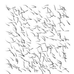
First results from new asemic glyph algorithm
That was way too busy, so I adjusted the space allocated to each glyph to they were better separated. The results were still disappointing: a weird snaky mess and not glyphlike at all.
Figure 22: Early results
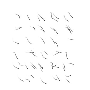
Early results from new asemic glyph algorithm
There now followed a cycle of pruning the set of control points and adjusting the stroke parameters: dozens of experiments, each running ten trials. I ended up separating the control points into several sets with different functions (starting versus ending points, for example). Then I added a randomizer that occasionally flipped control points to make things more interesting.
Figure 23: Tuned glyphs
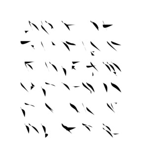
Tuned glyph shapes
The shapes didn't entirely look like glyphs, but they were pleasing and interesting and amenable to various stylistic experiments. Again a cycle of dozens of experiments with ten or so trials per experiment followed. Variations in colour. Variations in resolution. Latticing of the forms. Variation in the arrangement of the forms into meanders and circles.
Encapsulating the basic shapes into a component library function made creating these
variations easier. Each variant could use a path function to create a set of location
points, such as rectangular array, meander, or circle, and apply the glyph function
to create a glyph element at that location. Styling parameters adjust the overall
presentation. The art:glyph and art:stroke elements generate the appropriate SVG paths. Attributes provide some variations in
the presentation. For example, the attribute lattice enables or disables the latticing, and size allows for the rescaling of particular glyphs (seen in the circular variant). Stylesheet
parameters set default attributes for such attributes, allowing for more control.
Figure 24: Variations

Latticing
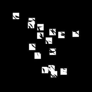
Meanders with latticing
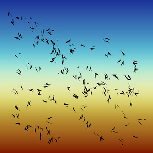
High resolution meanders

Circling
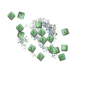
Textured
Variations on the glyph theme
Final Thoughts
The XML stack provides a good platform for generative art. Algorithmic experimentation can be separated from stylistic experimentation using domain specific languages. The use of domain specific languages lets us separate the details of SVG generation from the generative algorithms and use appropriate tools for each part. XQuery for algorithms, XSLT for transformation.
Using a declarative intermediate form for the works in a domain specific language allows for easier experimentation and better searchability. New works are often based on pieces from old works: having them as manifest components makes this easier. I can increase the artistic complexity without increasing the complexity of the main algorithms: the complexity is hidden in the components.
XQuery does lack some of the extensive libraries available in, say, Python or JavaScript. It does provide enough base functionality to be able to build up targeted libraries, such as the randomizer API. Specific implementations often have useful and interesting extensions which can be leveraged to good effect. Still, there is a lot of work to be done to build up basics. You want tessellate a Poincaré circle? Be prepared to do a lot of investigation and coding.
SVG seems verbose when you look at it, but it actually offers many higher level constructs (e.g. "ellipse"), and ends up being more compact than image formats such as JPEG. It allows arbitrary complex and structured information to be embedded invisibly, providing an excellent hook for tracking and searching.
Having a system for automatically tracking and embedding metadata about algorithm and rendering parameters and being able to override the parameters without editing code creates a virtuous circle, encouraging parameterization, which in turn encourages componentization.
The XML toolset — XQuery, XSLT, SVG — can be used to produce a variety of generative artworks. Enjoy!
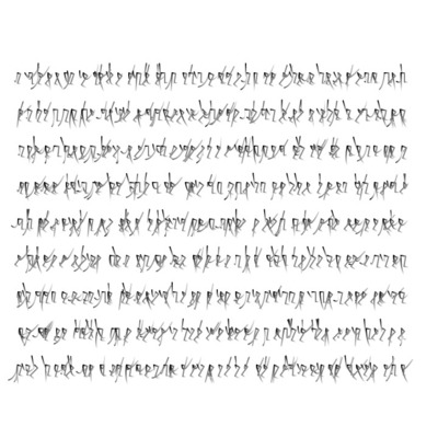
Asemic characters, non-spiral, generated with a Markov model of syllable structure, a Zipf distribution of glyphs, and a small amount of jittering in the angles
References
[SVN] Apache® Subversion, Apache Software Foundation. https://subversion.apache.org
[Boiroju12] Naveen Kuman Boiroju and M. Krishna Reddy, Osmania University. Generation of Standard Normal Random Numbers. InterStat, May 2012. http://interstat.statjournals.net/YEAR/2012/articles/1205003.pdf
[XML] W3C: Tim Bray, Jean Paoli, C. M. Sperberg-McQueen, Eve Maler, François Yergeau, editors. Extensible Markup Language (XML) 1.0 (Fifth Edition) Recommendation. W3C, 26 November 2008. http://www.w3.org/TR/xml/
[Crameri] Fabio Crameri, Scientific Colour Maps. https://doi.org/10.5281/zenodo.124386
[SVG] W3C: Erik Dahlström, Patrick Dengler, Anthony Grasso, Chris Lilley, Cameron McCormack, Doug Schepers, Jonathan Watt, Jon Ferraiolo, 藤沢 淳 (FUJISAWA Jun), Dean Jackson, editors. Scalable Vector Graphics (SVG) 1.1 (Second Edition) Recommendation. W3C, 16 August 2011. http://www.w3.org/TR/SVG11/
[Emacs] GNU Emacs, Free Software Foundation. https://www.gnu.org/software/emacs/
[Galanter03] Philip Galanter, Texas A&M. What is Generative Art? Complexity Theory as a Context for Art Theory. Available at http://www.philipgalanter.com/downloads/ga2003_paper.pdf.
[ImageMagick] ImageMagick®, ImageMagick Studio LLC. https://imagemagick.org/index.php
[XSLT] W3C: Michael Kay, editor. XSL Transformations (XSLT) Version 2.0 Recommendation. W3C, 23 January 2007. http://www.w3.org/TR/xslt20/
[MarkLogic] MarkLogic Server, MarkLogic Corporation. https://www.marklogic.com/product/marklogic-database-overview/
[DocBook] Bob Stayton. DocBook XSL: The Complete Guide, Fourth Edition. Sagehill Enterprises, 2007. http://www.sagehill.net/docbookxsl/index.html
[XQuery] W3C: Jonathan Robie, Michael Dyck, Josh Spiegel, editors. XQuery 3.1: An XML Query Language Recommendation. W3C, 21 March 2017. http://www.w3.org/TR/xquery-31/