Birnbaum, David J., and Ronald Haentjens Dekker. “Visualizing textual collation: Exploring structured representations of textual alignment.” Presented at Balisage: The Markup Conference 2024, Washington, DC, July 29 - August 2, 2024. In Proceedings of Balisage: The Markup Conference 2024. Balisage Series on Markup Technologies, vol. 29 (2024). https://doi.org/10.4242/BalisageVol29.Birnbaum01.
Balisage: The Markup Conference 2024 July 29 - August 2, 2024
Balisage Paper: Visualizing textual collation
Exploring structured representations of textual alignment
David J. Birnbaum
Professor Emeritus of Slavic Languages and Literatures
David J. Birnbaum is Professor Emeritus of Slavic Languages and Literatures,
University of Pittsburgh. Much of his electronic text work intersects with his research
in
medieval Slavic manuscript studies, but he also often writes about issues in the
philosophy of markup.
Ronald Haentjens Dekker
Researcher, DH Lab
Huygens Institute for the History of the Netherlands
Ronald Haentjens Dekker is a researcher and software architect at DHLab at the Huygens
Institute for the History of the Netherlands, part of the Royal Netherlands Academy
of
Arts and Sciences. As a software architect, he is responsible for translating research
questions into technology or algorithms and explaining to researchers and management
how
specific technologies will influence their research. He has worked on transcription
and
annotation software, collation software, and repository software, and he is the lead
developer of the CollateX collation tool. He also conducts workshops to teach researchers
how to use scripting languages in combination with digital editions to enhance their
research.
Copyright 2024 by the authors
Abstract
The goal of this report is to offer a contextualized introduction of the
alignment ribbon, a new visualization of textual collation
information, implemented in SVG. Textual scholars often align moments of agreement
and
moments of variation across manuscript witnesses in order to explore and understand
how
those relationships contribute to a theory of the text, that is, to
understanding the history of the transmission of a work. How to identify (an analytic
task),
model (an interpretive task), and communicate (a rhetorical task) the structural
relationships among witnesses are distinct but related aspects of the study of textual
transmission. We introduce the alignment ribbon as a contribution to the visual
representation of textual alignment.
The goal of this report is to offer a contextualized introduction of the
alignment ribbon, a new visualization of textual collation information,
implemented in SVG. The three main sections, sandwiched between this introduction
and a
conclusion, are:
About textual collation. Textual
scholars often align moments of agreement and moments of variation across manuscript
witnesses in order to explore and understand how those relationships contribute to
a
theory of the text, that is, to understanding the history of the
transmission of a work. The first major section of the present report provides an
overview
of collation theory and practice, which is the research context that motivated the
development of our new visualization and its implementation in SVG.
Modeling and visualizing alignment. Textual
collation is a research method that supports the study of textual transmission. Collation
is simultaneously an analytical task (identifying the alignments that facilitate an
insightful comparison of manuscript witnesses), a modeling task (interpreting those
alignments in a way that makes a theory of the transmission history accessible for
further
study), and a visualization task (translating the abstract model into a representation
that communicates the meaning to human readers). Textual collation is always about
text,
but visualizations can communicate features of the model through a combination of
textual
and graphic features. The second major section of this report surveys influential
visualization methods used in textual collation with the goal of identifying their
relative strengths and weaknesses. In particular, we provide a thorough history of
the
development of the variant graph, which has played a singularly prominent role in
collation theory and practice. The identification of the strengths and weaknesses
of
different visualizations matters because it motivates and informs the development
of our
original alignment ribbon visualization.
Alignment ribbon. The
alignment ribbon is an original collation visualization that seeks to combine the
textual
clarity of an alignment table with the graphical insights of variant-graph and storyline
visualizations. The alignment ribbon is implemented as the SVG output of a Scala program
that ingests plain-text input, performs the alignment, and creates the visualization.
The
output relies on SVG and SVG-adjacent features that are not always, at least in our
experience, widely used, and that enable us to produce the visualization we want without
compromise and without dependence on potentially fragile third-party visualization
libraries or frameworks. The third major section of this report describes the alignment
ribbon and its implementation, with particular attention to those SVG and SVG-adjacent
features.
About textual collation
This section introduces the research motivation and context for visualizing textual
collation. Subtopics explain why collation matters to textual scholars, how computational
philologists have engaged with machine-assisted collation in the past, and how our
current
work attempts to improve on previous implementations, including our own. Because it
would not
be appropriate or realistic to incorporate a comprehensive tutorial on textual collation
in
this report, this introductory section provides only a high-level overview of the
topic.
Textual collation relies on visualization in at least two different but overlapping
contexts. First (in workflow order), visualization can help ensure that the output
of a
collation process will be intelligible to the developers who must evaluate and measure
the
results of their implementation as they seek to improve it. Second, visualization
is one way
that end-user researchers can understand and communicate the results of the textual
analysis
that serves as the focus of their philological explorations. Visualizations tell a
story, and they are valuable for their ability to summarize complex information
concisely, a result that they achieve by, among other things, focusing attention on
some
features by excluding or otherwise deemphasizing others. This selectivity means that
every
visualization entails choices and compromises with respect to both what to include
and how to
represent it. It should not be surprising that different visualizations may be useful
for
different purposes, involving not only the different (even if overlapping) needs of
developers
and end-user philologists, but also diverse requirements within each of those
communities.
The terms collation and alignment are often used
interchangeably to refer to the organized juxtaposition and comparison of related
textual
resources. In this report we distinguish them, adopting the terminology of the Gothenburg
Model (see below), where alignment refers narrowly to the identification
of philologically significant moments of agreement and variation in textual resources
and
collation refers to a larger workflow that includes pre-processing to
assist in the alignment, the alignment itself, and post-processing to present the
alignment
results to the researcher in an accessible form.[1]
Why textual scholars care about collation
Philologists refer to manuscript copies of the same work as textual
witnesses, and it is rare for two witnesses to the same work to agree
in all details. If textual scholars were to discover four witnesses to the same work
that
agreed in most places, but where the moments of disagreement always fell into the
same
pattern (e.g., witnesses A and B typically share one reading at locations where witnesses
C
and D share a different reading), they would try to explain how those variants arose
as new
textual witnesses were created by copying (imperfectly) earlier ones. Absent specific
reasons to believe otherwise, a common and sensible working hypothesis is that one
of two or
more variant readings continues an earlier version of the text and other readings
have
diverged from it because they have incorporated deviations introduced, whether accidentally
or deliberately, during copying. Crucially, philologists assume, unless there is good
reason
to believe otherwise, that coincidences are unlikely to arise by chance, that is,
that the
scribes of A and B (or of C and D) did not independently introduce identical changes
in
identical places during copying. Willis 1972 (cited here from Ostrowski 2003, p. xxvii) explains the rationale for this assumption by means
of an analogy: If two people are found shot dead in the same house at the same time,
it is indeed possible that they have been shot by different persons for different
reasons,
but it would be foolish to make that our initial assumption (p. 14).
Variation during copying may arise through scribal error, such as by looking at a
source
manuscript, committing a few words to short-term memory, and then reproducing those
words
imprecisely when writing them into a new copy. Scribes may also intervene deliberately
to
emend what they perceive (whether correctly or not) as mistakes in their sources.
A scribe
copying a familiar text (such as a monk copying a Biblical citation in a larger work)
might
reproduce a different version of the text from memory. A scribe who sees a correction
scribbled into the margin by an earlier reader may regard it as correcting an error,
and may
therefore decide to insert it into the main text during copying. These are only a
few of the
ways in which variation may arise during copying, but whatever the cause, the result
is an
inexact copy. The witnesses that attest an earlier reading at one location will not
necessarily attest earlier readings at other locations; each moment of variation requires
its own assessment and decision. The is no justification in automatically favoring
the
majority reading because a secondary reading may be copied more than a primary one;
this
means that competing readings must be evaluated, and not merely counted. For reasons
explained below, there is also no justification in automatically favoring the oldest
manuscript; both older and younger manuscripts may continue the earliest readings.
Scholars who encounter textual variation often care about identifying the readings
that
might have stood in the first version of a work, which, itself, may or may not have
survived
as a manuscript that is available to the researcher. Textual scholars may also care
about
the subsequent history of a work, that is, about which changes may have arisen at
different
times or in different places across the copying tradition. The process of comparing
manuscript variants to construct an explanatory hypothesis about the transmission
of the
text is called textual criticism, and a necessary starting point for
that comparison involves finding the moments of agreement and disagreement among manuscript
witnesses. Identifying the locations to be compared closely across the manuscript
witnesses
is the primary task of collation.
Three challenges of collation
Collating a short sentence from a small number of witnesses is simple enough that
we can
perform the task mentally without even thinking about how the comparison proceeds.
Consider
the sentence below, taken from Charles Darwin’s On the origin of
species as attested in the six British editions published during the author’s
lifetime:
Table I
From Charles Darwin, On the origin of species
1859
The
result
of the
                              various,
quite
unknown,
or
dimly
seen
laws
of
variation
is
infinitely
complex
and
diversified.
1860
The
result
of
the
various,
quite
unknown,
or
dimly
seen
laws
of
variation
is
infinitely
complex
and
diversified.
1861
The
result
of
the
various,
quite
unknown,
or
dimly
seen
laws
of
variation
is
infinitely
complex
and
diversified.
1866
The
result
of
the
various,
quite
unknown,
or
dimly
seen
laws
of
variation
is
infinitely
complex
and
diversified.
1869
The
results
of
the
various,
unknown,
or
but
dimly
understood
laws
of
variation
are
infinitely
complex
and
diversified.
1872
The
results
of
the
various,
unknown,
or
but
dimly
understood
laws
of
variation
are
infinitely
complex
and
diversified.
The representation above is called an alignment table, and we’ll
have more to say about alignment tables as visualizations below. For now, though,
what
matters is that an alignment table models shared and different readings across witnesses
as
a sequence of what we call alignment points, represented by columns in
the table.[2] Alignment points can be described as involving a combination of
matches (witnesses share a reading), non-matches
(witnesses contain readings, but not the same readings), and indels
(insertions / deletions, where some witnesses contain readings and some
contain nothing). Because there may be more than two witnesses in a textual tradition,
these
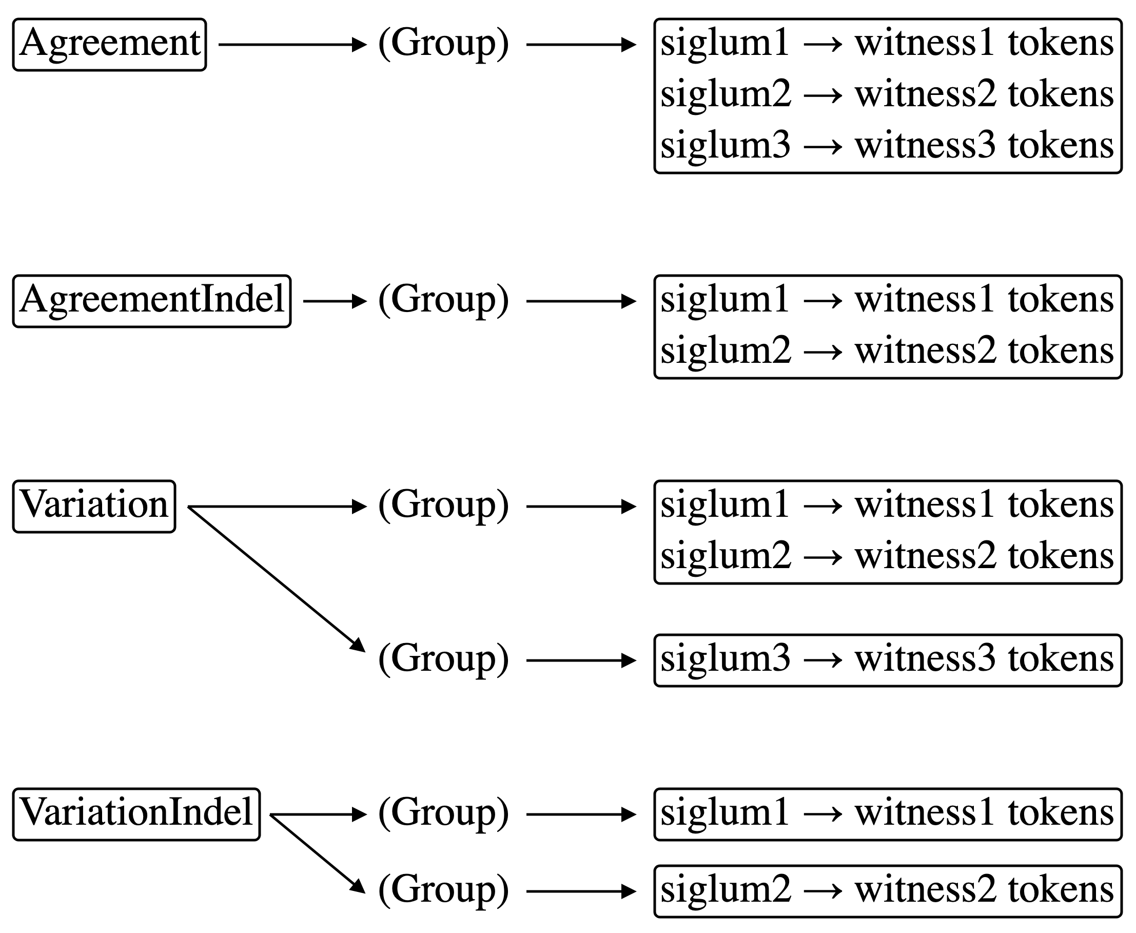
three types of pairwise relationships correspond to four full-depth
(all-witness) relationship types, which we call:
Agreement: All witnesses are present and have the
same value
AgreementIndel: Not all witnesses are present, but
those that are present all have the same value
Variation: All witnesses are present, but they do
not all have the same value
VariationIndel: Not all witnesses are present, and
those that are present do not all have the same value
It is easy to see in the alignment table example above that 1) the versions of this
sentence in the first four editions are identical to one another; 2) the same is true
of the
last two; and 3) the two subgroups agree with each other more often than not (all
witnesses
agree in fourteen of the nineteen textual columns). We happen to know the dates of
these
editions (something that is rarely the case with medieval manuscript evidence), but
even
without that chronological metadata we could hypothesize that the two subgroups go
back to a
common source (which explains the predominant agreement across the entire set of witnesses)
and that at each moment of divergence either one was created by editing the other
or both
were created by editing a common ancestor that is not available for direct study.
As those
options demonstrate, identifying the patterns of agreement and disagreement among
witnesses
is only part of the work of the philologist, who will also want to decide the direction
of
any textual transmission. In this case we have metadata evidence that the original
reading
is the one from the first edition (1859), which is reproduced without change in the
next
three (1860, 1861, 1866), and that Darwin then revised the text for the 1869 edition
and
reproduced those revisions in 1872. However, as mentioned above, comprehensive dating
information is rarely available with medieval manuscripts and we cannot be confident
that
the same witness or group of witnesses will always (that is, at all locations in the
text)
continue the earliest reading.
Most real-world collations do not tell as clear a story as the one above, and there
are
three types of common textual phenomena that pose particular challenges for aligning
textual
witnesses in order to understand the relationships among them:[3]
Repetition: The distribution of words in a text in
many languages converges, as the length of the text grows, on a distribution called
Zipf’s Law: [T]he most common word occurs approximately twice as often as the
next [most] common one, three times as often as the third most common, and so
on. (Zipf’s Law (Wikipedia); text in square brackets has been added) This
means that the repetition of words is to be expected, and part of the task of collating
textual witnesses involves choosing which instance of a repetition to align with which
other instances. In the alignment table above (Table I), the word
of occurs twice in each witness and it is easy (at least for a human)
to see which instances to align with which others. That decision is more challenging
when the number of repetitions increases and the amount of context around them does
not
tell as clear a story as the example above, where of occurs within the
three-word phrases result of the and
laws of variation.
Transposition: Scribes may change the order of
words (or larger units) while copying. For example, in another location Darwin writes
will be hereafter briefly mentioned in
the first four editions and will hereafter be
briefly mentioned in the last two. This is an adjacent transposition; transposition may also occur at a distance, such
as when an author moves a sentence or paragraph or larger section from one location
in a
work to another across intermediate text (which may or may not be shared by eome or
all
of the witnesses). Distinguishing actual editorial transposition from the accidental
appearance of the same content in different locations in different witnesses is further
complicated by repetition. We might expect editorial transposition (as contrasted
to the
accidental appearance of the same word in different contexts in different witnesses)
to
be more likely over short distances than long ones, but translating that vague truism
into rules that a computer can apply usefully can be challenging.
Number of witnesses: It is relatively easy to
compare two witnesses because the moments of comparison have only two possible outcomes:
assuming we have successfully negotiated repetition and transposition, the readings
at
each location are either the same or not the same.[4] Comparing three readings has five possible outcome groupings: three versions
of two vs one, one where all agree, and one where all disagree. Comparing four things
has fifteen possible outcomes: four versions of three vs one, three of two vs two,
six
of two vs one vs one (three groups), one with complete agreement and one with no
agreement. Even without expanding further it is easy to see that as the number of
witnesses increases linearly the number of possible groupings increases at a far greater
rate.[5] Computers often deal more effectively than humans with large amounts of
data, but the machine-assisted alignment of large numbers of long witnesses typically
requires heuristic methods because even with computational tools and methods it is
not
realistic to evaluate all possible arrangements and combinations of the witness
data.
The Gothenburg Model of textual collation
The Gothenburg Model of textual collation emerged from a 2009 symposium within the
frameworks of the EU-funded research projects COST Action 32 (Open scholarly
communities on the web) and Interedition, the output of which was the
modularization of the study of textual variation into five stages:[6]
Tokenization: The witnesses are divided into units
to be compared and aligned. Most commonly the alignment units are words (according
to
varying definitions of what constitutes a word for alignment purposes), but nothing
in
the Gothenburg Model prohibits tokenization into smaller or larger units.
Normalization: In a computational environment the
tokens to be aligned are typically strings of Unicode characters, but a researcher
might
regard only some string differences as significant for alignment purposes. At the
Normalization stage the collation process creates a shadow representation of each
token
that neutralizes features that should be ignored during alignment, so that alignment
can
then be performed by comparing the normalized shadows, instead of the original character
strings. For example, if a researcher decides that upper vs lower case is not
significant for alignment, the normalized shadow tokens might be created by lower-casing
the tokens identified during the Tokenization stage.[7]
Alignment: Alignment is the process of determining
which normalized shadow tokens in the different witnesses should be compared to one
another. It is the alignment process that identifies the moments of agreement and
moments of variation recorded in the columns of the alignment table example
above.
Analysis: Analysis refers to adjustments introduced
into the alignment after completion of the Alignment stage. These adjustments may
involve human intervention to resolve decisions that cannot be automated fully. More
interestingly, though, the Analysis stage refers also to automated adjustments. For
example, the Alignment stage of the current Python version of CollateX recognizes
agreement only when the normalized shadow tokens agree exactly, but that version of
CollateX also allows for near matching (that is, fuzzy matching).
Near matching is implemented as part of the Analysis stage, which means that it is
applied only to resolve alignment uncertainties that cannot be decided during the
preceding Alignment stage.
Visualization: Visualization might more accurately
be called output or serialization, since it
refers to outputting the result of the collation process for subsequent viewing (literal
visualization) or further downstream processing. CollateX supports several output
formats, including the alignment table illustrated above and others discussed
below.
One motivation for the development of the Gothenburg Model is that the work performed
by
the five components is likely to be important for any computational engagement with
textual
variation, but the way the different stages are implemented and applied may vary according
to language, text, and research question, as well as according to programming language
and
paradigm. The modular structure that constitutes the principal original contribution
of the
Gothenburg Model to collation theory and practice makes it possible to customize one
part of
the process without having to rewrite the others. In other words, the Gothenburg Model
regards collation as a processing pipeline, where the five stages
happen in order, the output of each serves as the input to the next, and no stage
has to
know about the inner workings of any other.[8]
The alignment of manuscript witnesses is an example of a more general process known
as
sequence alignment, which is well developed in bioinformatics, where
it is fundamental to comparing gene sequences. Although there are domain-specific
differences between textual and genetic sequencing (see Birnbaum 2020,
§1.2, p. 46 and Schmidt and Colomb 2009 §2.2, p. 500), the difference between
paired vs multiple-witness alignment is fundamental to both. Specifically, an algorithm
that
can be proven to create an optimal alignment of two sequences has been in use for
more than
fifty years (Birnbaum 2020 explores it within an XSLT context), but the
alignment of more than two sequences is considered to be an NP-hard problem, which
means—to
simplify—that no scalable (that is, implementable) algorithm is known that can ensure
the
optimal alignment of more than two witnesses.
The absence of an algorithm that ensures an optimal alignment of multiple witnesses
has
required work-arounds, the most common of which is progressive
alignment. Progressive alignment begins by aligning two witnesses (for which an
algorithm exists), regards that alignment as a sort of super-witness,
and then aligns it against a third witness, etc. One type of progressive alignment
begins by
merging two singleton witnesses and then incorporates the remaining witnesses into
the
mixture one by one. If the result of the initial merger of two singleton witnesses
is
modeled as a graph, subsequent mergers each combine one graph with one singleton.
We refer
to this as simple progressive alignment. A more powerful approach to
progressive alignment, which we call complex progressive alignment,
also permits mergers that do not involve any singletons, so that, for example, a first
step
might merge singleton witnesses A and B to create graph AB; a second step might merge
singleton witnesses C and D to create graph CD; and a third step might merge graphs
AB and
CD to create graph ABCD. The implementation of complex progressive alignment is more
challenging than implementing simple progressive alignment, and current release versions
of
CollateX (Java and Python) employ the simple type of progressive alignment, arriving
at an
alignment of all witnesses by incorporating one singleton at a time.
The reason progressive alignment is not wholly satisfactory is that, as a greedy
workflow, it is subject to order effects; once a super-witness has been
formed it cannot be broken apart, which means that progressive alignment may produce
different results according to the order in which the witnesses are incorporated.[9] This property is undesirable because the optimal alignment of multiple witnesses
from a philological perspective cannot depend on the order in which arbitrary researchers
at
an arbitrary moment happen to touch the witnesses. An alignment process might improve
the
outcome of progressive alignment by incorporating the witnesses in an order that reflects
the copying history, based on a heuristic scan and organization of the evidence into
a
guide tree, but the benefit of that strategy depends on the
informational quality of the scan, converging on a reductio ad absurdum
workflow that must perform and assess the quality of the entire computationally expensive
alignment with all possible permutations of the witnesses in order to determine the
optimal
order. More insidiously, because manuscript witnesses may incorporate and merge information
from multiple sources, the optimal order for incorporating witnesses into a progressive
alignment in one place may not be the optimal order in a different place.
What the collation of more than two witnesses requires, then, is
order-independent multiple-witness alignment, that is, a method that
considers all evidence from all witnesses simultaneously when making alignment decisions.
As
noted above, the current Java and Python versions of CollateX perform progressive
alignment,
and the authors of this report are in the process of implementing a new alignment
algorthm,
to be incorporated into a future release of CollateX, that will perform order-independent
multiple-witness alignment. Because order-independent multiple-witness alignment is
NP-hard,
our new method will necessarily rely on heuristics, including limited progressive-alignment
methods, but it is intended to reduce the susceptability of the alignment to order
effects,
even if it it not able to eliminate those effects entirely.
Our development of a new alignment algorithm provided a context for us to review both
the model underlying the way alignment is performed and recorded in CollateX and the
way the
results of the alignment process are exported and presented for visualization.
Modeling and visualizing alignment
The examination below of existing visualizations of textual alignment rests on the
following assumptions:[10]
Visualizations are selective views of data, which means that
different visualizations deliberately include and exclude different features and they
foreground different aspects of the features that they do include. Our discussion
below
does not attempt to identify the best visualization in any absolute way
because different visualizations may tell different useful stories about the same
original
data, and a visualization that is more effective when telling one story may be less
so
when telling another.[11]
The most useful data structures for modeling data to support
computational processing may not be the most useful for
visualization, that is, for telling a story to humans with visual
methods. For example, a model for processing may prioritize eliminating redundancy,
while
a visualization may deliberately include redundant information for rhetorical purposes.
The focus of our discussion below prioritizes the communicative
consequences of different visual expressions of the output of a collation process.
The same data structure may be expressed (serialized, represented) in different ways.
For example a graph can be understood mathematically as a set of
nodes (also called vertices) and a set of
edges (also called arcs), which means that a
graph can represented fully and correctly by listing the members of those sets. Such
lists
are not easy for humans to understand, and when we speak of graphs, we typically have
a
more … well … graphic image in mind. The graphic
renderings of variant graphs below (Variant graph)
use SVG to present the nodes and edges of a graph in ways that make the relationships
among them visually perspicuous. The discussion below explores the communicative
effects of different visual representations of variation.
Textual visualizations
Critical apparatus
The most familiar visualization of variation for philologists is likely to be the
critical apparatus, or apparatus criticus, a
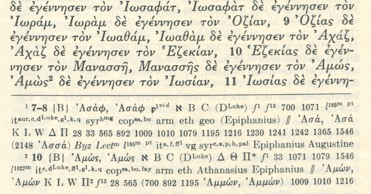
textual presentation that records variation across witnesses in notes (usually footnotes).[12] The image below of a critical apparatus is from the United Bible Societies
edition of the Greek New Testament:[13]
Figure 1: Greek New Testament (text and apparatus)
The continuous reading in larger print, at the top, represents the editors’ judgment
about the establishment of the text. This means that in situations
where the textual evidence is inconsistent, the editors represent, in the continuous
reading, what they believe is most likely to have appeared in a source ancestral to
all
surviving copies. The editors of this Greek New Testament do not regard any single
extant
manuscript as always attesting the best reading; that is, there is no
best witness. As a result, the main reading version does not
correspond to any single witness in its entirety, representing, instead, what is sometimes
referred to as a dynamic critical text.[14] Whether a particular work has a single extant best witness vs whether a
dynamic critical text is a better representation of the tradition is an editorial
decision.
Some editions that draw on multiple sources, especially where the chronology of the
editorial changes is known, may focus not on establishing an earliest text, but on
facilitating the comparative exploration of the evidence. The information from Darwin’s
On the origin of species displayed as an alignment table in Table I, above, is published digitally with a critical apparatus in
Barbara Bordalejo’s Online variorum of Darwin’s Origin of
species at
http://darwin-online.org.uk/Variorum/1859/1859-7-dns.html. Both the table
above and the online Variorum organize and present the readings from the six British
editions of the work published during Darwin’s lifetime. This type of evidence does
not
ask the editor to establish a dynamic critical text; the research question raised
by this
type of tradition and facilitated by a edition of multiple witnesses is not What is
likely to have stood in the original? (we know that the 1859 edition is Darwin’s
first publication of his text), but What did Darwin change in subsequent editions,
and when, and how should we understand those changes?[15]
The critical apparatus in the Nestle-Aland New Testament is
selective, that is, it reports only variants that the editors
consider significant for understanding (and, in the case of the
United Bible Societies publication, translating) the text. Reasonable persons might
disagree, at least in places, about what constitutes significant vs insignificant
variation, about which see below.[16] Furthermore, the apparatus mentions explicitly only readings that disagree
with the editors’ preferred reading; this is called a negative
apparatus, and it implies that any witness not listed in the apparatus agrees
with the reading in the critical text. A negative apparatus that conforms to this
assumption is informationally equivalent to a positive apparatus, that is, one that
explicitly lists the witnesses that agree with the preferred reading. These and other
parsimonious editorial preferences may be unavoidable in the case of the Greek New
Testament, which is preserved in and attested by an unmanageably large number of witnesses.[17]
Understanding a critical apparatus is challenging for new users because the notational
conventions prioritize concision, but editions come with introductions that explain
the
meaning of the manuscript identifiers (called sigla) and other
special editorial conventions. In the example above, the second apparatus entry
(introduced by a small, superscript numeral 2) says that, with respect to
verse 10, there is some degree of doubt (the B in curly braces is on a scale from virtual certainty for
A to a high degree of doubt for
D) about the decision to select ᾽Αμώς, ᾽Αμὼς as the preferred reading (in the last two lines of the main
text); that ᾽Αμώς, ᾽Αμώς is attested in witnesses
א, B, C, etc.; that witnesses K,
L, W, etc. attest
instead ᾽Αμών, ᾽Αμών; and that witnesses 700, 892, and 1195 attest ᾽Αμμών, ᾽Αμμών,
which the editors regard as a variant spelling of the version with a single μ.
The critical apparatus has long been the predominant method of reporting textual
variation in paper publication; it is valuable for its extreme concision, which is
especially important, for economic reasons, in the context of publication on paper.
Additionally, because a critical apparatus groups sigla that share a reading, it
foregrounds which witnesses agree with one another at a particular moment in the text.
The
concision is undeniably cognitively alienating for new users, but philologists quickly
become reasonably comfortable with it, at least when working with texts with which
they
are familiar. At the same time, the critical apparatus as a representation of textual
transmission comes with at least two severe informational limitations:
Editors typically record only what they consider textually significant variants in
an apparatus. Removing distractions that do not contribute to understanding the
history of the text has obvious communicative merit, but what happens when reasonable
persons disagree about what constitutes significant vs insignificant variation? The
complete omission from the apparatus of variation that the editor considers
insignificant makes it impossible for users to assess and evaluate the editor’s
decisions and agree or disagree with them in an informed way. It is, to be sure, the
editor’s responsibility to make critical decisions that interpret the evidence for
users, but the complete exclusion of some variants as insignificant is a different
editorial action than deciding which version goes into the main reading text and which
versions are relegated to the apparatus as variants. Ultimately, excluding variants
that some readers might reasonably consider textually significant even when the
editors do not compromises the documentary value of the edition. Furthermore, in the
(common) case of a negative apparatus, the omission of a witness from the apparatus
becomes ambiguous: either an omitted witness agrees with the preferred reading in
all
details or it disagrees with it, but in a way that the editor regards as not
significant. Insofar as editions sometimes rely on manuscript evidence that is not
otherwise easily accessible to users, an editor’s decisions about the omission of
variants are not verifiable.
For many the principal goal of an edition is to establish an authoritative text,
that is, one that reconstructs (or, perhaps more precisely, constructs a hypothesis
about) the earlier contents of the text by eliminating changes that were introduced,
whether accidentally or intentionally, during copying.[18] The critical apparatus prioritizes its focus on deviation from a
hypothetical best text at individual moments by gathering the variants for such
moments in separate critical annotations. That focus serves the purposes of
foregrounding the preferred readings and documenting variation, but one side-effect
is
that it becomes challenging to use the edition with the goal of reading a particular
witness consecutively, since the text of that witnesses is sometimes in the apparatus
and sometimes implicitly in agreement with the main text.
Digital editions based on a critical apparatus can mitigate this complication by
allowing the reader to select any witness as a copy text (a primary witness, presented
continuously in its entirety, in the place of a dynamic critical text) and display
readings from other witnesses as variants. This approach can be seen in, for example,
Darwin online (see p. 1 at
http://darwin-online.org.uk/Variorum/1859/1859-1-dns.html) and the
Frankenstein Variorum (see p. 1 at
https://frankensteinvariorum.org/viewer/1818/vol_1_preface/).
The centuries-long tradition of recording variation in a critical apparatus ensures
that it will continue to be the preferred representation for some philologists, especially
if their focus is on presenting a hypothesis about what is likely to have stood in
an
original text. At the same time, digital editions remove the economics of paper
publication from an assessment of the costs and benefits of the concision afforded
by the
critical apparatus. A critical edition requires a record and representation of variation,
but those do not have to be expressed in a traditional, footnoted critical apparatus.
Ultimately the critical apparatus is one of several available ways of representing,
for
human perception and understanding, information about textual variation.
Alignment table
Overview
As explained above, an alignment table is a two-dimensional table that displays the
full contents of all witnesses in intersecting rows and columns, where each cell
contains either text or nothing. In Table I, above, each row
contains all of the words from one witness to the textual tradition and the columns
represent alignment points, that is, the columns align words that the editors regard
as
corresponding to one another across witnesses. If a witness has no reading at a
particular location in the tradition the cell for that witness in that column is
empty.
An alignment table, such as Table I above, avoids at least
two of the limitations of a footnoted critical apparatus:
As noted above, reading the full text of a specific witness continuously from
start to finish is challenging with a critical apparatus because some of the text
is
reported implicitly in the main reading text (that is, only because of the absence
of any explicitly reported variant), while other text appears in footnoted apparatus
entries. Reading a specific witness continuously from this type of edition therefore
requires the reader to reassemble the continuous text mentally by identifying and
piecing together snippets of the main text and pieces recorded as variants.
Furthermore, because the footnoted apparatus prioritizes grouping the sigla of
witnesses that share a reading, there is no stable place where a reader can expect
to find the variants (if any) that belong to a particular witness. This
fragmentation and inconsistency imposes a heavy cognitive load on readers who want
to focus their attention on a particular witness.
Unlike a critical apparatus, an alignment table makes it easy to read the
continuous text of any individual witness by reading across a row. There is no
ambiguity about where to look for the text of a particular witnesses; all text (or
gaps in the text) in a specific witnesses will always appear, in order and
continuously, in a predictable row.
A limitation of an alignment table that arises as a consequence of making it
easy to read the continuous text of any witness is that an alignment table does not
represent patterns of agreement among witnesses as clearly as a critical apparatus,
which groups the sigla that share a variant. With a small number of witnesses, as
is
the case with the six editions in Table I, above, it is not
difficult to understand at a glance the agreements and disagreements. But especially
because different agreement patterns mean that witnesses that agree will not always
appear in adjacent rows in an alignment table, recognizing those groupings imposes
increasing cognitive costs as the number of witnesses grows.
As also noted above, a critical apparatus typically includes only what the
editor considers significant variants, which means that a reader cannot know, in the
absence of any record of variation, whether there is no variation at a location or
whether there is variation but the editor does not regard it as significant.[19] An alignment table, on the other hand, provides the full text of all
witnesses, and therefore is naturally able to record variation whether the editor
considers it significant or not. This enhances the documentary value of the edition
and enables readers to form their own assessments of individual moments of
variation, which is not possible in a selective apparatus-based edition that omits
entirely variant readings that the editor considers insignificant.
At the same time, an apparatus-based edition with a dynamic critical text, such as
the continuous reading text above the apparatus in our example from the Greek New
Testament (Figure 1), always reports explicitly the
readings that the editor prefers in situations involving variation. That reporting
is
not automatic in an alignment table that records only the readings from the witnesses,
since that sort of table lacks a dynamic record of the editor’s interpretation of
moments of variation. For that reason, if an alignment table is to record an editor’s
interpretation of variation, it must add that interpretation as a supplement to the
transcriptions of the witnesses. This feature is discussed below.
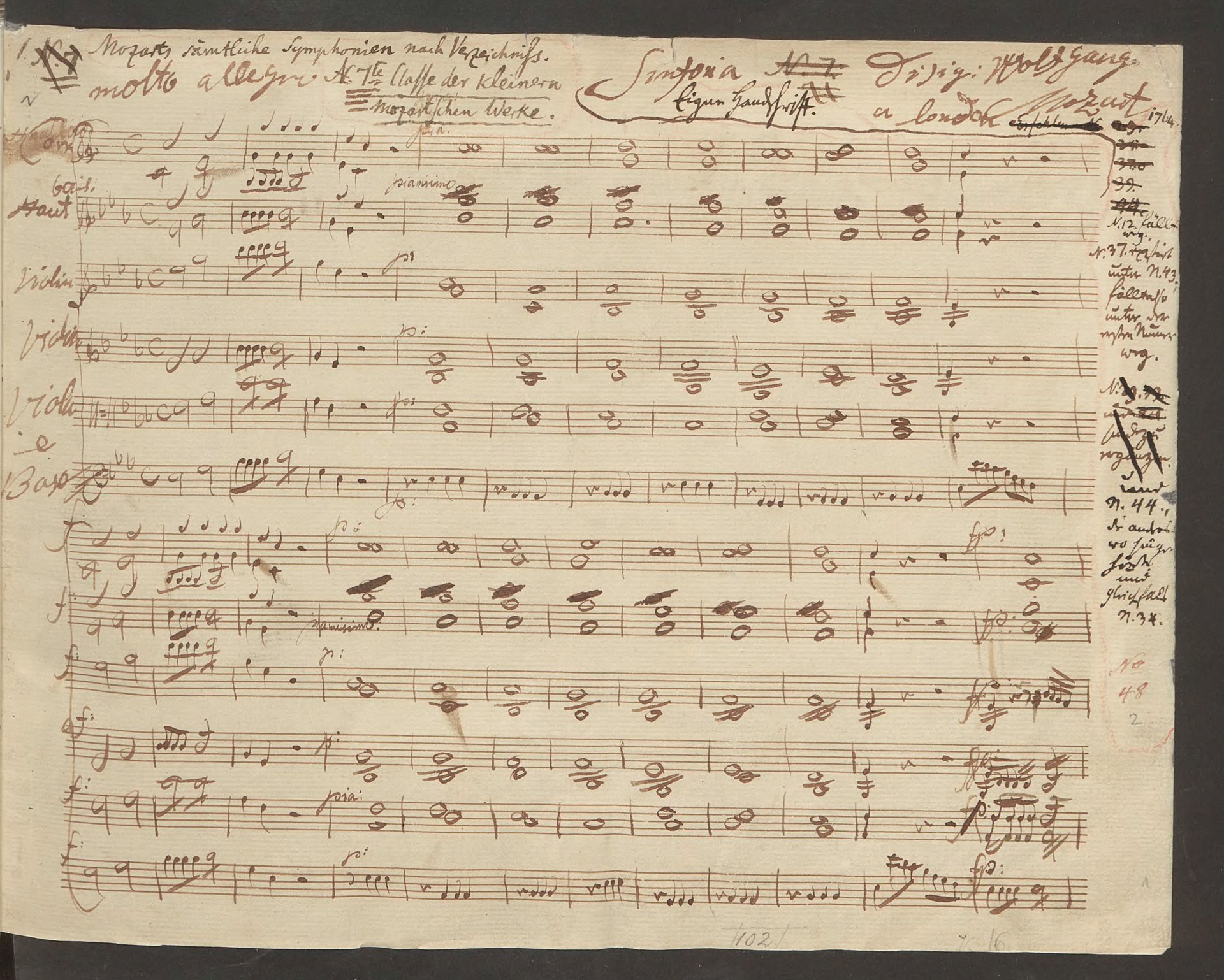
An edition published as an alignment table, such as Ostrowski 2003, is sometimes called an interlinear collation or a
Partitur (German for musical score) edition, where the
synchronized presentation of the text of all witnesses in parallel rows resembles
a
conductor’s orchestral score, which represents the different instrumental parts in
parallel rows and aligns the measures in columns according to where parts are sounded
together. The first image below is the beginning of an autograph manuscript of Mozart’s
Symphony No. 1 in E♭ Major (K. 16):[20] The second is from the online edition of Ostrowski 2003.[21]
Figure 2: Mozart Symphony No. 1 in E♭ Major (K. 16), autograph manuscript
Both of these visualizations use rows to represent parts (instruments for Mozart,
manuscripts and editions for Ostrowski 2003) and columns to represent
alignments.
Swapping rows and columns in alignment tables
In the discussion and examples above we describe rows as representing witnesses and
columns as representing alignment points, but nothing in the concept of the alignment
table prevents the editor from reversing that layout, so that each witness occupies
a
particular column and the alignment points are represented by the rows. If we swap
the
rows and columns of Table I, the result looks like the
following:
Table II
From Charles Darwin, On the origin of species
1859
1860
1861
1866
1869
1872
The
The
The
The
The
The
result
result
result
result
results
results
of
of
of
of
of
of
the
the
the
the
the
the
various,
various,
various,
various,
various,
various,
quite
quite
quite
quite
unknown,
unknown,
unknown,
unknown,
unknown,
unknown,
or
or
or
or
or
or
but
but
dimly
dimly
dimly
dimly
dimly
dimly
seen
seen
seen
seen
understood
understood
laws
laws
laws
laws
laws
laws
of
of
of
of
of
of
variation
variation
variation
variation
variation
variation
is
is
is
is
are
are
infinitely
infinitely
infinitely
infinitely
infinitely
infinitely
complex
complex
complex
complex
complex
complex
and
and
and
and
and
and
diversified.
diversified.
diversified.
diversified.
diversified.
diversified.
These tables are informationally equivalent and each has advantages and
disadvantages. In the case of digital editions of texts that are written in a
left-to-right writing system, such as Darwin’s English-language On the origin
of species, tension arises between the naturalness of placing each witness
in its own row, to support continuous left-to-write reading (Table I), and the fact that after a fairly small number of words the
display must either scroll horizontally (which users notoriously find less comfortable
than vertical scrolling[22]) or wrap blocks of text that consist of several lines.[23] Arranging the witnesses in columns mitigates these limitations, but not
without introducing its own complications:
As long as the number of witnesses is not large, arranging the witnesses in
columns removes the need for horizontal scrolling, which is desirable from the
perspective of the user experience (UX). Some editions, though, will require more
witnesses than can comfortably be displayed across the screen without horizontal
scrolling, which means that arranging the witnesses in columns is not a universal
remedy for the inconvenience of horizontal scrolling.
One disadvantage of arranging the witnesses as columns is that it changes the
word-to-word reading direction. In the case of the Darwin example, we are used to
reading English-language texts horizontally, moving our focus down and to the left
margin only when no more room remains on the current horizontal physical line.
Arranging the witnesses in columns narrows those physical lines, with the result
that reading a specific witness entails reading individual words horizontally while
reading consecutive words entirely vertically. This is a not a familiar layout for
reading English-language texts continuously.
Reducing repetition in alignment tables
An alignment table, whatever its orientation, involves a large (and often very
large) amount of repetition. Unnecessary repetition during data
entry creates opportunities for user error and unnecessary repetition in
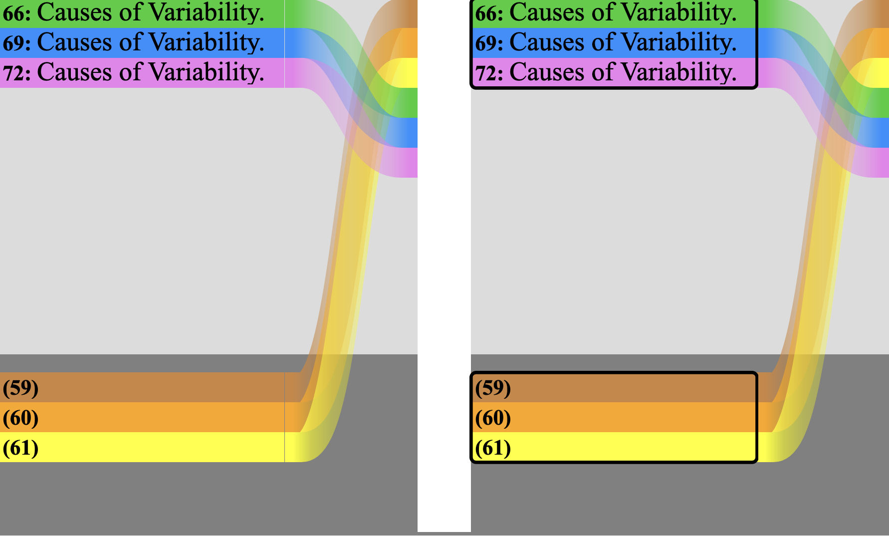
information modeling increases storage space.[24] At the same time, repetition is not necessarily undesirable for
communicating information, and the focus of this report is
primarily on visualization, and not on modeling or processing. Users most naturally
recognize pieces of information as related when they are physically close to one another,[25] when they are similar in some way,[26] and when they appear inside the same boundary or container.[27] For these reasons, repeating words in each witness in an alignment table
where they occur makes it easier in some ways for readers to perceive and understand
the
content of the individual witnesses.
It is possible in some circumstances to remove repetition in an alignment table by
merging cells where adjacent witnesses contain the same readings. Table III, below, is informationally equivalent to Table II, above, but it removes variation by merging cells
horizontally where witnesses share a reading.
Table III
From Charles Darwin, On the origin of species
1859
1860
1861
1866
1869
1872
The
result
results
of
the
various,
quite
unknown,
or
but
dimly
seen
understood
laws
of
variation
is
are
infinitely
complex
and
diversified.
An obvious limitation of this approach is that it is not possible to merge cells
that are not adjacent to one another. In Table III all
readings that are shared by witnesses happen to be shared by witnesses that are adjacent
in the table (and adjacent chronologically, since the columns are arranged by date
of
publication), but On the origin of species also contains readings
that are shared by witnesses that are not chronologically consecutive. There is no
consistent ordering of the six editions in the tables above that would make all shared
readings adjacent, and repeatedly changing the order of the columns to manipulate
the
adjacency would introduce unwanted cognitive friction by undermining the reader’s
spatial memory.[28]
Tokenization and alignment tables
The first stage of the Gothenburg Model, Tokenization, is where
the witness texts are divided into units to be aligned. The default tokenization in
the
release versions of CollateX separates tokens at sequences of whitespace (that is,
divides the text into orthographic words) and also breaks off boundary punctuation
marks
into their own tokens. Users can override this default. The three Darwin tables above
use a custom tokenization rule that separates the text into words on whitespace but
does
not break off boundary punctuation into its own token, so that, for example, the text
of
all witnesses ends with the single token diversified., which includes a
trailing dot, instead of with a sequence of the token diversified (without
the dot) followed by the token . (just a dot).
Separating the input texts into words during tokenization does not require that the
words be reported individually at the fifth and final Gothenburg stage, called
Visualization[29]. CollateX supports a process that it calls
segmentation, which merges adjacent alignment points that share
alignment properties. For example, all witnesses in our Darwin example have the same
first token (The) and same third through fifth tokens (of the
various,), but there are differences in the second token (result
vs results) and the sixth (quite in four witnesses and nothing
in the other two). With segmentation activated, Table I would
look like:
Table IV
From Charles Darwin, On the origin of species
1859
The
result
of the various,
quite
unknown, or
dimly
seen
laws of variation
is
infinitely complex and diversified.
1860
The
result
of the various,
quite
unknown, or
dimly
seen
laws of variation
is
infinitely complex and diversified.
1861
The
result
of the various,
quite
unknown, or
dimly
seen
laws of variation
is
infinitely complex and diversified.
1866
The
result
of the various,
quite
unknown, or
dimly
seen
laws of variation
is
infinitely complex and diversified.
1869
The
results
of the various,
unknown, or
but
dimly
understood
laws of variation
are
infinitely complex and diversified.
1872
The
results
of the various,
unknown, or
but
dimly
understood
laws of variation
are
infinitely complex and diversified.
The point of segmentation is that an open alignment point ends and a new one begins
not with every new token, but only when the agreement pattern among witnesses changes.
In this example the alignment-point columns alternate between those that show full
agreement (columns 1, 3, 5, 7, 9, and 11) and those that show variation or indel
situations (columns 2, 4, 6, 8, 10). It will not always be the case that columns will
alternate in this way; for example, if there are two adjacent alignment points that
both
show variation, but with different patterns of agreement among witnesses, the two
will
be output consecutively.
An alignment table with segmentation can arrange the witnesses either in rows, as
in
Table IV, above, or in columns, as in Table V, below:
Table V
From Charles Darwin, On the origin of species
1859
1860
1861
1866
1869
1872
The
The
The
The
The
The
result
result
result
result
results
results
of the various,
of the various,
of the various,
of the various,
of the various,
of the various,
quite
quite
quite
quite
unknown, or
unknown, or
unknown, or
unknown, or
unknown, or
unknown, or
but
but
dimly
dimly
dimly
dimly
dimly
dimly
seen
seen
seen
seen
understood
understood
laws of variation
laws of variation
laws of variation
laws of variation
laws of variation
laws of variation
is
is
is
is
are
are
infinitely complex and diversified.
infinitely complex and diversified.
infinitely complex and diversified.
infinitely complex and diversified.
infinitely complex and diversified.
infinitely complex and diversified.
Regardless of the orientation of the table, it is also possible (with this example,
but not universally) to combine the merged or shared readings with segmentation, as
in:
Table VI
From Charles Darwin, On the origin of species
1859
1860
1861
1866
1869
1872
The
result
results
of the various,
quite
unknown, or
but
dimly
seen
understood
laws of variation
is
are
infinitely complex and diversified.
As we said earlier, merging cells where witnesses share a reading is possible only
with adjacent cells, which means that it is a useful visualization only where all
shared
readings are shared by consecutive witnesses. That pattern occurs in the example above,
but it it not the case elsewhere in On the origin of
species.
Single-column alignment table
A modification of the alignment table to deal with fact that shared readings can be
merged visually only when the witnesses are adjacent in the table is the
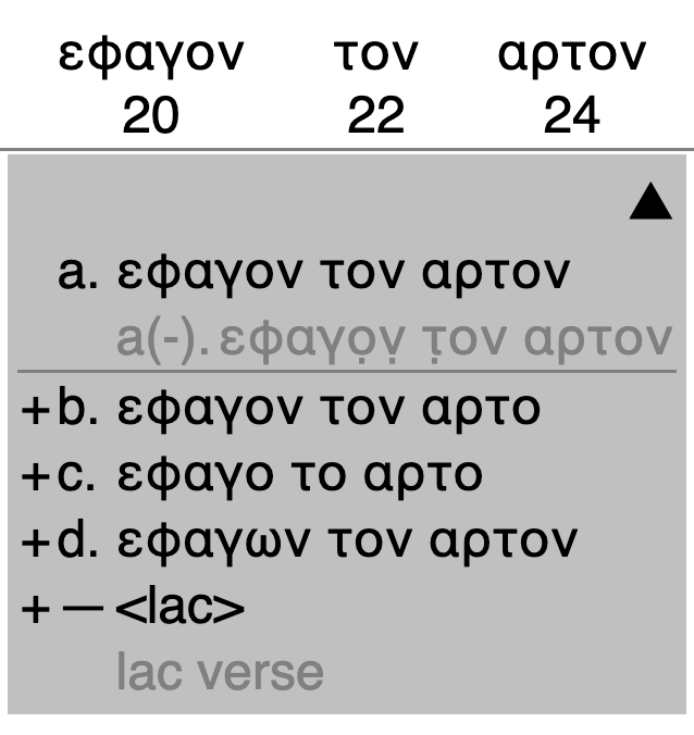
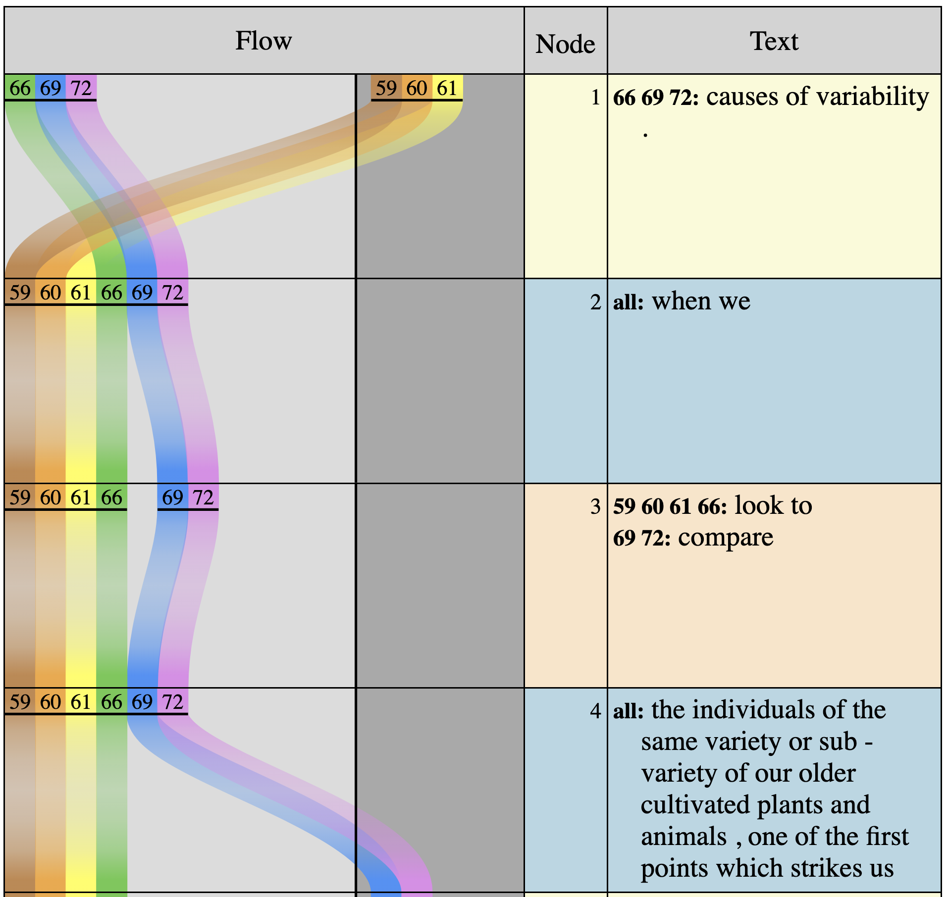
single-column alignment table. This visualization divides the
output the same way as the segmentation examples, above—that is, it starts a new
alignment point when the pattern of agreement among witnesses changes. As the name
implies, though, instead of rendering different witnesses in their own columns and
merging adjacent ones, it displays the readings for an alignment point in a list within
a single column, e.g.:
Table VII
From Charles Darwin, On the origin of species
No
Readings
1
All: The
2
1859, 1860, 1861, 1866: result
1869, 1872: results
3
All: of the various,
4
1859, 1860, 1861, 1866: quite
1869, 1872:
5
All: unknown, or
6
1859, 1860, 1861, 1866:
1869, 1872: but
7
All: dimly
8
1859, 1860, 1861, 1866: seen
1869, 1872: understood
9
All: laws of variation
10
1859, 1860, 1861, 1866: is
1869, 1872: are
11
All: infinitely complex and
diversified.
The organization of the Readings column looks familiar because it is identical to
a
positive critical apparatus in that it groups and records the readings of all witnesses,
and not only those that diverge from the editor’s preferred reading. In this case,
for
reasons discussed above, there is no dynamic critical text, and although we could
select
a copy text (such as the first edition as chronologically primary
or the last as Darwin’s final, and therefore most experienced, expression of his ideas),
there is no lost original to imagine and (re)construct. With that said, if we were
to
select one witness as primary, to be presented consecutively, the Readings column
could
be synchronized with it automatically and rendered as either a positive critical
apparatus (as is) or a negative critical apparatus (by removing the sigla for the
copy
text and witnesses that agree with it from the apparatus entries).
We found the single-column alignment table useful during development because it
provided the same information about an individual alignment point as we would find
in a
row of Table VI, except that the
single-column alignment table could also record the agreement of witnesses that were
not
consecutive in chronological or any other consistent order, which is a feature that
cannot be expressed in an alignment table. At the same time, although the single-column
alignment table provides a useful representation of a single alignment point, it is
difficult to read consecutively. All of the information needed to reconstruct the
full,
continuous text of any witness is present, but because of unpredictable layout and
gaps
in witnesses, the visual flow through a single witness is inconsistent, interrupted,
and
distracting. Insofar as the single-column alignment table is ultimately just a positive
critical apparatus without a main text, it is not surprising that it reproduces the
challenges of using a critical apparatus to read a single witness continuously, and
it
does so without the continuous and legible critical text that accompanies a traditional
critical apparatus.
The best text in an alignment table
Unlike with critical apparatus layout, which foregrounds the editor’s assessment of
the best reading by placing it—and only it—in the main text, the transcription and
interlinear publication of all witnesses does not automatically include an editorial
judgment about which reading to prefer at moments of variation. To incorporate editorial
assessment, and not just transcription, into an interlinear collation editors can
include, in parallel with the actual textual witnesses, their own determination of
a
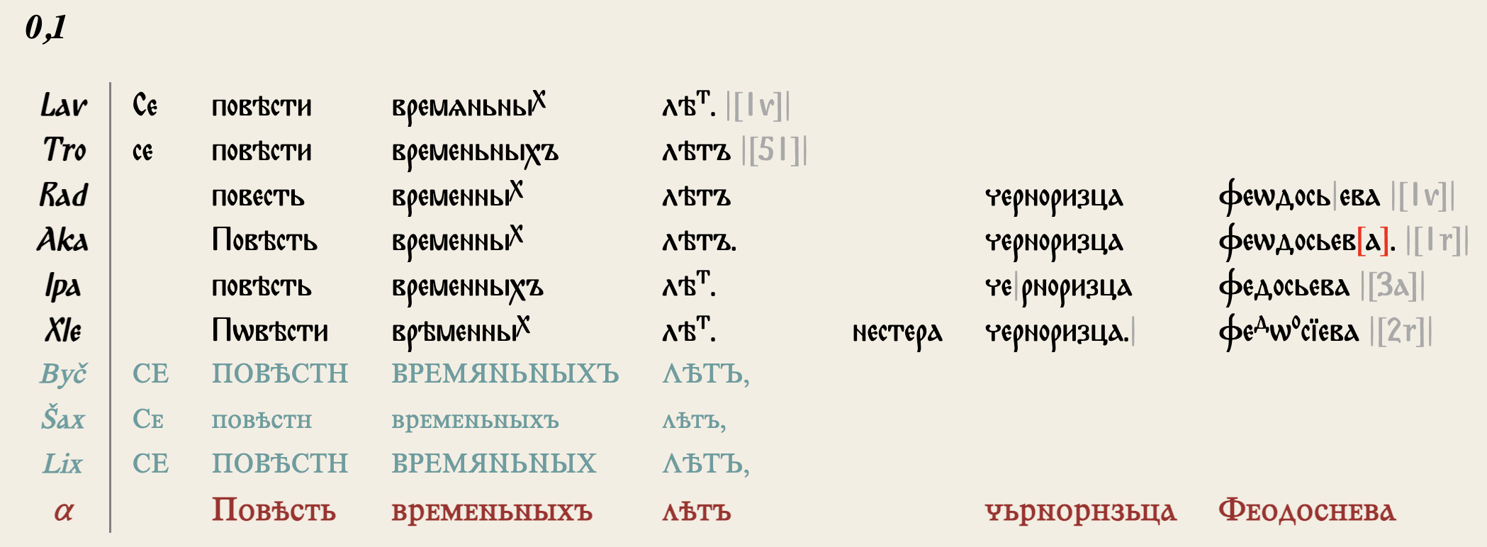
best reading. In Figure 3 (from Ostrowski 2003), above, the black rows represent transcriptions from
manuscript witnesses, the red row at the bottom represents the editor’s dynamic critical
text, and the blue rows represent critical texts published by other editors. This
arrangement makes it easy to see at a glance where the witnesses agree or disagree
with
one another, which readings the editor considers most authoritative at each location,
and how other editors evaluated the same variation to arrive at their decisions about
which readings should be incorporated into the critical text.
An interlinear edition overcomes many of the intellectual and cognitive limitations
of a critical apparatus, but at the expense of being practical only with a fairly
small
number of witnesses because the difficulty of seeing the patterns of agreement grows
as
the number of witnesses in the edition increases. A related consideration, at least
with
respect to paper publication, is that an interlinear collation incorporates a large
amount of repetition or redundancy, which increases the size (and therefore also the
production cost) of the edition. For example, the paper edition of Ostrowski 2003, with approximately ten witnesses and editions, fills three
volumes that contain a total of approximately 2800 8-1/2 x 11 pages and occupy
approximately eleven inches of shelf space.[30]
Redundant repetition is sometimes regarded instinctively as undesirable because by
definition it contributes no information that is not already available in a different
form. In the case of visualization, though, repetition that may be informationally
redundant may nonetheless contribute to the rhetorical effectiveness of the edition.
For
that reason, repetition is not automatically a weakness that should be avoided
in a visualization; it is, instead, a communicative resource with costs and benefits
that must be assessed on their own terms.
Alignment table summary
Ordering challenges: Even when the number of
witnesses is not large, an interlinear collation raises questions about how to order
them. On the one hand, ordering the witnesses identically throughout the edition enables
the reader to memorize their relative and absolute positions quickly, avoiding the
cognitive friction that would arise from having to read the sigla carefully at every
line to verify which readings go with which witnesses. On the other hand, it would
be
easier to see which witnesses share readings if those witnesses were adjacent to one
another, and in that case the groupings (that is, the grouping-dependent orders) might
vary at different locations in the edition. We find consistent order easier to
understand, even when it means that not all shared readings will be rendered in adjacent
or merged cells. In Ostrowski 2003, for example, the witnesses observe
a consistent order and are grouped according to overall patterns of agreement suggested
by a stemma codicum, even though that means that sometimes
witnesses that share readings may be separated from one another visually by text from
other witnesses.[31]
Repetition challenges: An alignment table that does
not merge witnesses, and that instead repeats readings for each witness in which they
appear (such as Table I, above), makes it easy to read any
individual witness continuously. At the same time, not merging adjacent cells where
witnesses share a reading means that the reader has to determine at every alignment
point which witnesses agree with which others. How easy that is depends on the visual
similarity of the readings. For example, readings of different lengths may be recognized
easily as different, while readings of the same length may require closer inspection
and
consideration.
Separating the recording of variation from its
evaluation: Insofar as an alignment table contains an affirmative statement
about what each witness says (or doesn’t say) at every alignment point, it avoids
the
selectivity that can prevent readers from forming their own assessments of an editor’s
decision about whether two witnesses attest a significant difference. The continuous
text above a critical apparatus necessarily presents a privileged reading, either
as a
dynamic critical text or as a best witness selected as a copy text. Because an alignment
table presents a legible continuous view of every witness, it does not automatically
have a single privileged text (whether a dynamic critical text or a best witness).
The
editor of an alignment table may incorporate a dynamic critical text by entering it
alignment point by alignment point, in parallel with the witness data, as in Figure 3.
Comparing alignment tables and critical apparatus:
Our (somewhat subjective) experience has been that:
An alignment table makes it easy to read the continuous text of any witness, but
harder to see which witnesses agree or disagree at a particular location. A critical
apparatus makes it easier to see the patterns of agreement and variation, but harder
to read any the text of witness continuously except the base text.
With a small number of witnesses an alignment table is more informative and
easier to understand than a critical apparatus.
Both a critical apparatus and an alignment table quickly become difficult to
read and understand as the number of witnesses increases, but an alignment table
becomes challenging sooner than a critical apparatus. Because an alignment table is
much more verbose than a critical apparatus, it also becomes impossible to represent
on a single screen or page much sooner than is the case with a critical
apparatus.
Graphic visualizations
Variant graph
The model used internally for recording the alignment of witnesses in current releases
of CollateX is based on the variant graph, a structure popularized in
Schmidt and Colomb 2009 after having been introduced almost half a century
earlier. An SVG representation of the variant graph is also the principal graphic
output
format available in CollateX.
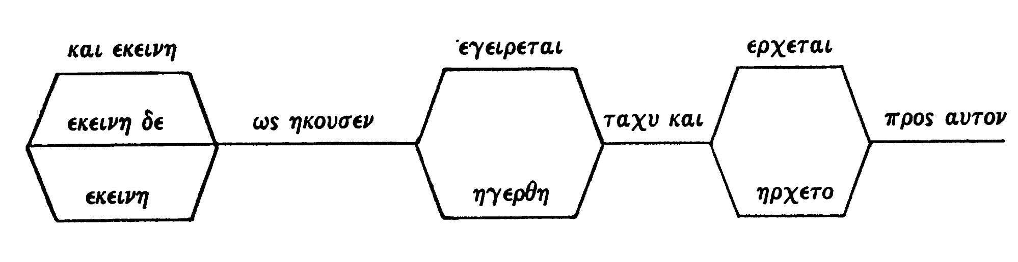
The earliest discussion of the variant graph as both model and visualization of
which we are aware is Colwell and Tune 1964, which appears not to have
been cited subsequently in relevant literature until its rediscovery by Elisa Nury
and
Elena Spadini (Nury and Spadini 2020, p. 7), who reproduce the example
below:
Figure 4: Variant graph (Colwell and Tune 1964, p. 254)
Colwell and Tune 1964 uses the term
variation-unit to describe a location where not all witnesses
agree.[32] Their illustration records the text of the readings on what graph theory
would call the edges, with no information recorded on the nodes. The discussion in
their
article leaves no doubt that they are also tracking, for each variation-unit, which
readings are attested in which witnesses, although they do not include witness
identifiers in their illustration.
Our term alignment point, discussed above, is not the same as
the Colwell and Tune 1964 variation-unit because an alignment point
includes both locations with variation and locations where all witnesses agree, while
the variation-unit in Colwell and Tune 1964 refers only to locations where
witnesses diverge. In Figure 4, then, there are three
variation-units but six alignment points. The focus on locations with variation matters
in Colwell and Tune 1964 because the authors propose that variation-units
be counted to explore and assess relationships among witnesses, and most of their
article focuses on principles for classifying and evaluating types of variant readings
as part of the text-critical process.[33]
The next appearance of the variant graph that we have been able to locate is Sperberg-McQueen 1989, which is also mentioned in passing in Nury and Spadini 2020 (p 7, fn 19). Sperberg-McQueen 1989
does not include any images (the write-up originated as a two-page conference abstract),
but it describes the confluence and divergence of readings as analogous to the branches
of a river delta, adopting the label Rhine Delta for the model. The
illustration below shows how the Rhine (and Meuse) split into multiple channels, some
of
which may then merge or continue to divide:
Annual average discharge of the Rhine and Meuse 2000-11
Under the term Rhine Delta, Sperberg-McQueen introduces many
features and properties of the variant graph that serve as the focus of later work
by
others:
In this non-linear model, the multiple versions of a text are imagined not as so
many parallel, non-intersecting lines, but as curves that intersect, run together
for
a while, and then split apart again, like the channels in a river delta. Unlike the
channels of most river deltas, the versions of a text often merge again after
splitting. The data structure takes its name from one riverine delta where such
reunion of the channels does occur; I have christened it the Rhine
Delta structure. Unlike the two-dimensional model of complex texts, this
structure stores passages in which all versions agree only once; it is thus more
economical of space. It also records the agreements and divergences of manuscripts
structurally, which makes the task of preparing a critical apparatus a much simpler
computational task.
Formally, the Rhine Delta structure is a directed graph, each node of which is
labeled with one token of the text and with the symbols of the manuscripts which
contain that token. Each arc linking two tokens is labeled with the symbols of the
manuscripts in which the two tokens follow each other. There is a single starting
node
and a single ending node. If one follows all the arcs labeled with the symbol of a
specific manuscript, one visits, in turn, nodes representing each token of that
manuscript, in sequence. Passages where all the manuscripts agree are marked by nodes
and arcs bearing all the manuscript symbols. Passages where they disagree will have
as
many paths through the passage as there are manuscript variants.
It can be shown that from this structure we can, for any variant, produce all the
conventional views of linear text and perform all the usual operations (deletion,
insertion, replacement, travel, search and replace, block move, etc.). Moreover, we
can readily generate the various conventional views of complex texts: base text with
apparatus, texts in parallel columns, text in parallel horizontal lines. Unlike other
methods of handling textual variation, the Rhine Delta has no computational bias
toward any single base text state; the user pays no penalty for wishing to view the
text in an alternate version, with an apparatus keyed to that version. (Sperberg-McQueen 1989)
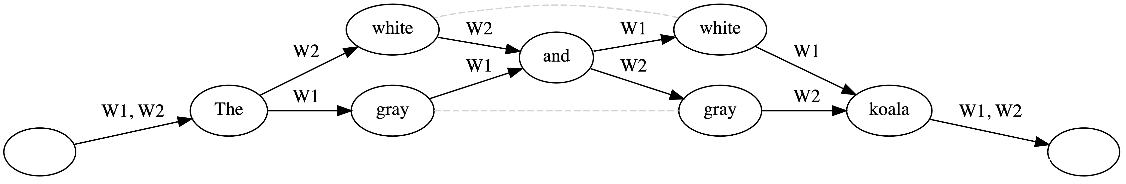
The Rhine Delta model as described in Sperberg-McQueen 1989 records textual readings and witness identifiers on
nodes and witness identifiers (alone) on edges, which is also the way information
is
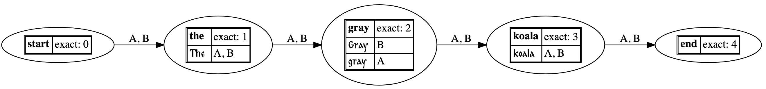
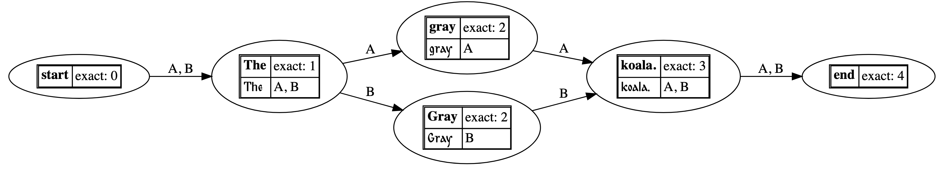
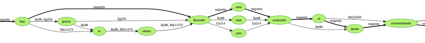
allocated among nodes and edges in CollateX.[35] The following image is part of the CollateX variant-graph visualization of
the data in Table I, but see also the excerpt from Documentation (CollateX) below, which explains how this visualization does not, in
fact, expose all token information:
As far as we can tell, Sperberg-McQueen 1989 appears not to have
been discussed in any detail in the literature until the author republished the full
text of the abstract himself on his own website after hearing a conference presentation
that described a model with very similar properties. Sperberg-McQueen 1989 explains that:[36]
This work came to mind recently when I heard the paper A Fresh
Computational Approach to Textual Variation by Desmond Schmidt and Domenico
Fiormonte at the conference Digital Humanities 2006, the first International
Conference of the Alliance of Digital Humanities Organizations (ADHO), at the Sorbonne
in Paris earlier this month. So I have unearthed the abstract and put it on the
Web.
The abstract of the 2006 ADHO presentation by Schmidt and Fiormonte mentioned above
was published as Schmidt and Fiormonte 2006, where the authors describe
and illustrate a variant graph structure that they call a
textgraph. The following image is from p. 194 of that conference
abstract:
Figure 7: Textgraph (Schmidt and Fiormonte 2006, p. 194)
The first use we have been able to find of the term variant
graph is in Schmidt and Colomb 2009, which presents the same
general model as Schmidt and Fiormonte 2006, but in greater detail and
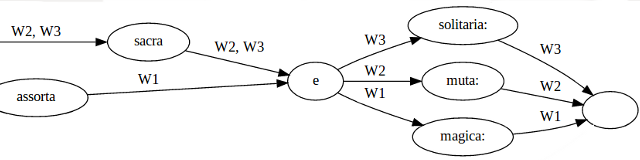
with more explanation. The following variant graph image is from Schmidt and Colomb 2009, p. 510:
Figure 8: Variant graph (Schmidt and Colomb 2009, p. 510)
Schmidt and Colomb 2009 emphasizes many of the same appealing features
of the variant graph as a model as Sperberg-McQueen 1989: it reduces
redundancy (see, for example, the extensive repetition in Table I), it permits the concise representation of textual editing operations (§3.4, pp.
503–04), and it supports specific computational operations on the graph itself (reading
a single version, searching a multi-version text, comparing two versions, determining
what is a variant of what, and creating and editing (§5, pp. 508–10)). The algorithm
in
Schmidt and Colomb 2009 for creating and editing a variant graph is
progressive in the sense in which that term is traditionally used in multiple-sequence
alignment, that is, it incorporates one singleton witness at a time into the
graph.
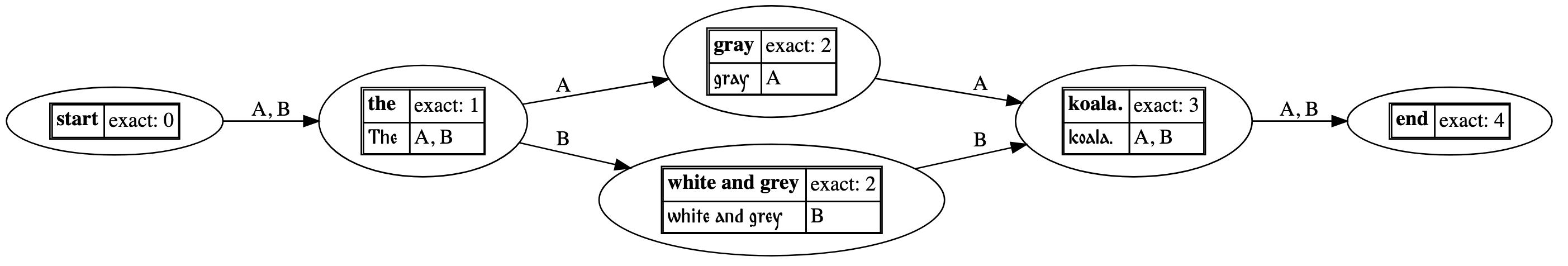
The representation of the variant graph in Schmidt and Colomb 2009
puts both textual content and witness identifiers on the edges of the graph. The Start
and End nodes, indicated by circled S and E, represent the
starting and ending point of a traversal. There is exactly one path from start to
end
for each witness, which can be traversed by following the edges labeled for that
witness. The dotted lines represent transposition edges; they function as references
(the gray text is a copy of the black text with which it is connected by a tranposition
edge) and are not part of any traversal.
As mentioned above, the CollateX variant graph, similarly to the earlier Rhine Delta
model and unlike the model in Schmidt and Colomb 2009, stores the tokens
that contain textual readings on the nodes of the graph, and the only information
that
the Rhine Delta model and CollateX store on the edges is witness identifiers. Schmidt and Colomb 2009 do not mention this difference; the lone reference to
Sperberg-McQueen 1989 in Schmidt and Colomb 2009
reads, in its entirety:
Such a structure is intuitively suited to the description of digital text, and
something like it has been proposed at least once before in this context, but was
abandoned apparently because it could not be efficiently expressed in markup
(Sperberg-McQueen, 1989).
It is possible to transform either of the two representations (text on nodes vs text
on edges) to the other automatically, which means that they can be implemented in
ways
that are informationally equivalent, but the difference nonetheless merits attention
from a software-engineering perspective; see the discussion below.
CollateX was developed under the auspices of the EU Interedition research program
in
2009, with Ronald Haentjens Dekker and Gregor Middell as the two project leads. (About (CollateX)) Middell brought Schmidt and Colomb 2009 to
Haentjens Dekker’s attention (neither developer knew about Sperberg-McQueen 1989 at the time), they recognized the variant graph as a
useful model of textual variation, and they modified what they found in Schmidt and Colomb 2009 to move the tokens off the edges and onto the nodes.
Insofar as edges in graph theory express relationships between nodes, putting no
information on the nodes and all information on the edges would reduce the nodes to
nothing but meeting places for edges, with no information or properties of their own,
which makes the meaning of the nodes opaque.[37] But the developers of CollateX also had a more specific reason for putting
the witness content on the nodes: the tokens that represent witness content in CollateX
are complex objects with multiple properties, and not just string values. As Middell
explains in Documentation (CollateX) (text in square brackets has been
added):
In order to account for the separation of concerns laid out above [the five stages
of the Gothenburg Model], CollateX’[s] implementation of Schmidt’s model adjusted
the
latter slightly. Instead of labelling the edges of a variant graph with two
attributes—the content as well as the sigils [witness identifiers] of text versions
containing it—the edges of variant graphs in CollateX are only labeled with sigil
sets. The version’s content segments—in the form of partial token sequences—have been
moved to the nodes/vertices. The ending of the example graph then looks like this
(with sigils being mapped from A, B, C to W1, W2, W3):
CollateX’[s] Variant Graph Model
The above illustration does not reveal the internal structure of the graph
completely insofar as the nodes’ labels in this figure are a simplification. For
instance, the second node in the graph (read from left to right) is labeled
sacra, with the two versions W2 and W3 sharing some
content. More precisely though and in line with the above definition of
tokens and their equivalence relation, W2 and W3 do not share some
content. Instead they both contain a token with the content
sacra, both deemed to be equal according to the definition of a
specific token comparator function. In the graphical representation of the variant
graph above, this subtle distinction is not made and both tokens are just represented
via their common textual content. In CollateX’[s] data model though, this distinction
is still relevant and represented: Each node/vertex in a variant graph is not modelled
via textual content (as it would be the case when translated directly from Schmidt’s
model) but as a set of tokens per node originating from one or more versions, with
all
tokens in such a set belonging to the same equivalence class.
The described change to Schmidt’s model serves mainly two purposes: Firstly, it
allows for arbitrary tokens to be compared and their commonalities, differences as
well as their sequential order to be represented in a graph structure. Secondly,
CollateX’[s] graph model is easy to transform into the tabular representation
introduced further above by ranking the graph’s nodes in topological order and
aligning tokens which belong to nodes of the same rank.
Where transpositions occur (not in the example above), the CollateX variant graph
represents them with dotted lines. This corresponds to a similar special type of edge
between nodes that contain the same textual content in Schmidt and Colomb 2009, where it is represented by a dashed line (see the
example at Figure 8). The use of a special type of edge
avoids cycles when traversing the graph according to its principal edges.
The variant graph as a visualization in CollateX
The utility of the variant graph in modeling has been confirmed
by the successful use of CollateX in projects, where the variant graph functions as
the
internal model of the result of the alignment process, which can then be rendered
visually as a graph (as in Figure 6, above) or
transformed into an alternative visualization format (such as the alignment table
in
Table I, above). The focus of the present report, however, is
not on the variant graph as a model, but on its utility as a
final-form graphic visualization that communicates alignment and
variation information to end-users.
Any visualization of variation, including the textual (and pre-digital) critical
apparatus, becomes difficult to read as the extent of the variation grows, and both
the
critical apparatus and the variant graph manage the volume of information with the
help
of methods that we can usefully compare to data compression. Both visualization and
data
compression are transformations of a data set that retain something that matters for
a
particular purpose while excluding details that don’t matter for that purpose. As
the
name implies, the purpose of data compression is creating an output file that is smaller
(as measured in bytes) than the non-compressed input. The visualization of data
typically (although not obligatorily) aims for a smaller
presentation size. Smaller presentation in the case of a critical
apparatus might entail including only variation that the editor considers significant
and choosing a negative apparatus over a positive one. In the case of graphic
visualization, the editor includes only selected information with the goal of fitting
into a small space (such as a single screen or page) a representation of just what
the
editor considers important (for a particular purpose) about the data.
Data compression methods are commonly categorized as either
lossless or lossy, where the difference is
that the exact original data can be restored from lossless—but not from
lossy—compression. A critical apparatus that includes only variation that the editor
considers significant is lossy because it excludes—completely and
irretrievably—information that end-users might consider important. Insofar as a critical
edition is often used as a surrogate for original data sources, especially when original
manuscript data is not easily available to users of the edition, variation that an
editor regards as insignificant is not documented and not recoverable. Choosing a
negative apparatus instead of a positive one, on the other hand, is lossless because
a
negative apparatus comes with an implicit default: the editor asserts that any witness
not recorded explicitly in an apparatus entry agrees at that location in all significant
features with the continuous reading text (whether dynamic critical text or copy text
based on a favored manuscript).
Visualization in general is typically not intended to present (or enable the
recovery) of all features of an original set of data. Researchers use visualization
to
tell a story (that is, in the case of textual collation, to
communicate a theory of the text) by including some properties
while omitting others, so that the properties needed for the communicative purpose
will
stand out clearly. For example, as the discussion of the CollateX variant graph above
explains, a node in the CollateX variant graph contains not just plain textual
characters (the string rendered inside an ellipse in the visualization), but a set
of
tokens, which are complex objects with multiple properties. The simplification in
this
variant-graph visualization is lossy because all properties except the normalized
string
value of the token are discarded and the string is represented once regardless of
the
number of aligned tokens with which it is associated, which makes the graph easier
to
read.
CollateX actually supports two variant-graph visualizations, a simplified one that
silently merges tokens that share a normalized reading and a more information-rich
one
that performs the merge but also renders information about differences among original,
non-normalized forms of the tokens. Consider the following collation input:
Look, a koala!
Look, Koala!
Look, a gray koala!
The witnesses all begin with the same two tokens (Look,
,) and end with the same token (!), but the tokens in
the middle vary. Note especially that witnesses A and C contain the token
koala (lower-case k), which an editor would align with
Koala (upper-case K) in witness B. If we tell CollateX
to normalize the tokens by ignoring case before performing alignment, the basic (simple)
variant-graph visualization silently merges koala
with Koala:
Figure 10: CollateX basic variant-graph output
With CollateX configured to ignore case differences during alignment, the basic
variant-graph output silently merges lower-case koala with upper-case
Koala
The rich variant-graph output from CollateX performs the same merge because we’ve
told it that case differences should not be treated as significant during alignment.
CollateX nonetheless retains its knowledge of those differences even while not letting
them affect what it merges, and the rich variant-graph visualization exposes
them:
With CollateX configured to ignore case difference during alignment, the rich
variant-graph output also merges lower-case koala (witnesses A, C)
with upper-case Koala (witness B), but in this version the output
exposes the original differences among the non-normalized tokens
The basic visualization is easier to read because less ink means less competition
for the reader’s attention, and the main thing we see is where readings are considered
the same for alignment purposes. As is often the case, easier to read
entails a cost, which in this case is the suppression and concealment of differences
that the editor considers insignificant for alignment purposes, but that might
nonetheless be regarded as important in other contexts.
CollateX normalization is controlled by end-users, and although case-folding may be
a very common type of normalization, it isn’t the only type. When working with a heavily
inflected language, for example, a researcher might want to align on lemmatized forms,
ignoring inflectional differences in order to focus on lexical differences by excluding
grammatical ones. Birnbaum 2015 describes the implementation of a
Soundex-like strategy for aligning texts in a heavily inflected language with unstable
orthography, and Birnbaum and Eckhoff 2018 describes a strategy for
aligning Greek and Old Church Slavonic texts by normalizing them to (only) part of
speech, that is, aligning nouns with nouns, verbs with verbs, etc., as in the following
example (reformatted from an image on p. 12):
Figure 12: Multilingual alignment with CollateX
Alignment of Greek and Old Church Slavonic by part of speech. Solid edge lines
apply to both languages, dotted lines only to Greek, and dashed lines only to Old
Church Slavonic
The developers in this case customized the variant graph output format in Figure 12 to render only the original,
non-normalized string values of the tokens, but the tokens contained additional
properties. In particular, they incorporated a part-of-speech property, which served
as
the shadow normalization used to perform the alignment, which the developers chose
to
exclude from the visualization because it was not important for understanding the
texts.[38]
Excursus: Informational differences between variant graphs and alignment
tables
The variant graph model in CollateX includes all information
about tokens, alignment, and variation. As we write above, a
visualization—unlike the model—typically does not include all
information because the purpose of a visualization is to tell a story, not all data
is
relevant for every possible story, and irrelevant data in a visualization is clutter
that
makes the story harder to understand. For that reason, even the rich variant-graph
visualization in CollateX does not, by default, expose all properties of nodes. User
requirements cannot always be predicted, and the modular nature of the Gothenburg
Model
means that if neither of the built-in CollateX variant-graph visualizations (simple,
rich)
corresponds adequately to their requirements, users can create their own
alternatives.
It is possible to render any information from the variant-graph model (that is, any
information about tokens, alignment, and variation) in a variant-graph visualization,
but
there is information in the model that cannot be expressed in an alignment-table
visualization. Two types of information that cannot be represented in an alignment
table
are discussed below.
An alignment table, which must align all tokens, neutralizes groupings that are
present in a variant graph
A variant graph represents the alignment of corresponding tokens from different
witnesses by placing the tokens on the same node. An alignment table represents that
same type of alignment by placing the tokens in the same column. A single column in
an
alignment table, however, does not always correspond to a single node in a variant
graph; it corresponds to what we called an alignment point above. That is, a column
represents an alignment of all witnesses—including some with completely unrelated
readings and some with no readings (represented by empty cells)—at a particular location
in the alignment. In addition to putting readings from a shared variant-graph node
in
the same column, an alignment table puts readings from different variant-graph nodes
in
the same column when they have the same rank in the variant graph,
where rank means that [e]ach node is assigned a higher rank than the highest
ranked node that point[s] to it. (Wernick 2017; text in
square brackets is added).[39] For that reason, an alignment table is not able to distinguish readings from
different witnesses that are in the same column because they were on the same node
in
the variant graph model from those that were on different nodes of the same rank.
Consider, for example, an alignment of The gray koala with The
Gray koala (note the case difference). When Normalization is configured to
ignore case differences, the middle word is stored on the same node in the variant
graph:
Figure 13: Rich variant graph with case folding
The neutralization of case differences during the Normalization stage means that
gray and Gray are on the same node
However, when case differences are not neutralized for alignment purposes the
readings gray and Gray are stored on different nodes that
have the same rank:
Figure 14: Rich variant graph without neutralization of case
If case differences are not neutralized during the Normalization stage
gray and Gray are on different nodes, but the nodes
have the same rank in the graph
The two different variant graphs above nonetheless correspond to the same alignment
table, with gray and Gray aligned within the same
column:
Table VIII
Same alignment table either with or without the neutraliztion of case
differences
A
The
gray
koala
B
The
Gray
koala
The relationship of gray to Gray is self-evident, and
it’s easier to see from other examples why putting readings into the same column of
an
alignment table because their nodes have the same rank is a blunt tool. For example,
the
method would just as easily align The gray koala with The
prehistoric koala or The toy koala (neither of which is a koala
at all). What gray and Gray have in common is lexical
identity, but that isn’t why they wind up in the same column. What they also have
in
common, and the only thing that gray and prehistoric and
toy have in common, is that they happen to appear in the same context.
This relationship is what we called a non-match above, it is a meaningful part of
the
alignment result, and the alignment table renders it correctly. Our point is that
in
doing so, the alignment table must neutralize a distinction that is not neutralized
in a
variant graph.
If we think of the columns of an alignment table as representing the alignment
points that we defined earlier, an alignment table does a poor job of representing
groups of readings within an alignment point. Readings that share a node (by virtue
of
evaluating as equal according to a comparison of their normalized properties) can
be
considered to form a group, while those that share a rank but not a node may wind
up at
the same rank only because of properties of their neighbors. As we noted in our
discussion of alignment tables, above, rows with readings that share a node are not
necessarily even adjacent to one another; an alignment table is not designed to
represent groupings within a column. This means that expressing a variant-graph model
as
an alignment-table visualization entails a loss of grouping information.
The fact that CollateX assigns witness readings to columns according to node rank
in
the variant graph model creates a challenge when there are gaps in a witness. Consider
the following witness data:
The gray koala.
The white and grey koala.
The first (one) and last (two) tokens of the witnesses match, but the remaining
middle token in Witness A, gray, does not match any of the three middle
tokens in Witness B exactly (note that gray in Witness A is spelled
differently than grey in Witness B). The variant graph output of CollateX
for this alignment is:
Figure 15: Variant graph without an exact match
The variant graph shows the different paths for Witnesses A and B without
aligning all tokens and without representing the absence of readings
explicitly
Editors might disagree about how best to transform this variant graph into an
alignment table visualization, but it is unlikely that any editor will prefer the
default alignment table created by CollateX:
Table IX
Undesirable default alignment by rank in variant graph
A
The
gray
koala
.
B
The
white
and
grey
koala
.
The reason CollateX defaults to an alignment table layout that most editors would
consider suboptimal is that the CollateX default settings have no understanding of
closest match. This reflects an engineering decision: finding a
closest match is both unnecessary in most cases and much more expensive computationally
than finding an exact match, which means that it would not be realistic to make it
the
universal behavior during the Alignment stage of the Gothenburg Model. Correspondences
that can be described with simple algorithms, such as case differences, can be
neutralized easily during the Normalization stage, at which point CollateX can look
for
exact matches across normalized values without additional computational cost. In
principle users could create a Normalization function that would neutralize the
distinction between gray and grey, but because the
difference is lexically idiosyncractic (e.g., we would not want to normalize
pray and prey the same way), implementing this sort of
function would require considerably more developer time and effort than implementing
case-folding.
Users who agree in their dislike of Table IX might disagree about
what they would prefer to see in its stead. One option would be to align
gray with grey, as in:
Table X
Alignment of variant spellings
A
The
gray
koala
.
B
The
white
and
grey
koala
.
Users can ask CollateX to produce the alignment table above (Table X) by switching on the near matching option, which aligns tokens
according to the closest match only when two conditions are satisfied: 1) there is
no
exact match and 2) there is a gap in the shorter witness.[40] Near matching creates a non-traversal near-matching
edge in the variant graph, which is used to adjust the rank of the nodes,
which in this case produces:
Figure 16: Variant graph with near matching
Turning on near matching creates a non-traversal near-matching
edge that is interpreted as overriding the default ranking algorithm to
assign the same (higher) rank to nodes connected by a near-matching edge.
Assigning the same rank to nodes causes their readings to be rendered in the same
column in a corresponding alignment table because assignment of a node to a column
in
CollateX is controlled by rank. What makes near matching tractable in this situation
is
that it is invoked during the Analysis (not Alignment) stage of the Gothenburg Model
and
only when the two conditions mentioned above are met. That situation arises rarely
enough that the limited use of near matching does not impinge noticeably on the overall
performance.
A different user option might be to align gray with the complex
phrase white and gray, as in:
Table XI
CollateX alignment table with segmentation
A
The
gray
koala.
A
The
white and grey
koala.
The user can invoke this behavior by switching on segmentation,
which collapses adjacent nodes along a path in the variant graph as long as the edge
labels (the witness identifiers) do not change. Turning on segmentation creates a
different variant graph, one with fewer nodes, and the node with gray in
Witness A winds up in the same column as white and grey in Witness B
because the nodes have the same rank in the graph:
Figure 17: Variant graph with segmentation
With segmentation switched on, the tokens white and grey in
Witness B are assigned to the same node in the graph, which maps to Table XI as an alignment table because the nodes in the middle
have the same rank
Reasonable persons might disagree about whether the version with segmentation above
(Table XI) offers a better alignment than the one with near
matching (Table X). Ultimately, we would not expect automated
collation to identify a single best alignment in situations where human editors might
prefer different alignments for different reasons. CollateX accommodates different
user
preferences by incorporating switches that put these decisions under user control.[41]
We’ve devoted a lot of attention above to complexities involved in expressing a
variant graph model as an alignment table because the underlying issue is that there
cannot be an unambiguous, round-trippable relationship between a variant graph and
an
alignment table because a variant-graph visualization tells a different story about
alignment than an alignment table.[42] The variant graph in Figure 15
does not strictly align gray with any one of the three tokens in the
other witness because the exact position of a node on a variant-graph path is not
informational (as long as the order of the nodes does not contradict the order of
the
text in the input documents). What the variant graph model does record is that the
path
from The to koala for Witness A passes through a single
node and the one for Witness B passes through three nodes (in a specific order). The
CollateX visualization of a variant graph has to plot the gray node of
Witness A somewhere, and by default it does that according to the rank of the node
in
the graph, but the location of a node along a path is a rendering artifact that is
not
part of the information value of the variant-graph model. This differs from the meaning
of a column in an alignment table; when the CollateX alignment table assigns nodes
with
the same rank to the same column, that decision does acquire an informational meaning
because the meaning of a column in an alignment table is that all cells in the column
correspond to one another for alignment purposes. The correspondence may happen because
the tokens are evaluated as having the same value (after the Normalization stage)
for
alignment purposes (in which case they are on the same node) or it may happen because
they are on different nodes that have the same rank (whether originally or because
of
near matching). In some cases correspondence because of shared rank may reflect a
complete non-match, where non-matching tokens wind up sandwiched between matching
ones,
as in The gray koala vs The other koala; we refer to this
as a forced match because the readings are forced into the same
column by their neighbors, who leave them nowhere else to go.
The upshot of this difference is that tokens that share a column in an alignment
table are presented as aligned, and because every token must appear in exactly one
column and every witness must be represented by either a token or a gap in every column,
an alignment table asserts an explicit alignment for every token or gap in each witness
with either a token or a gap in every other witness. A variant graph, on the other
hand,
represents readings as associated only when they share a node and, differently, when
they are connected by a near-matching edge. In other situations a variant graph makes
no
explicit assertion about the relationship of readings in one witness to readings in
other witnesses. This means that a variant-graph visualization, but not an alignment
table, can represent the difference between readings that share a node and readings
on
different nodes that share a rank.
A variant graph (but not an alignment table) can represent transposition and near
matching
The term transposition describes a situation where witnesses
cannot align all matching nodes simultaneously because corresponding nodes in different
witnesses are ordered differently. Consider:
The gray and white koala
The white and gray koala
These witnesses have exactly the same tokens, but because an alignment cannot
rearrange the order of tokens within a witness, CollateX cannot align both
white with white and gray with
gray. The current CollateX Java release (although not the Python one)
is able to render information about transposition in the variant-graph
visualization:
Figure 18: Variant graph with transpositions
The dashed lines represent non-traversal transposition
edges, which connect nodes that are transposed with respect to each
other
If we ask CollateX to create an alignment table from this variant graph it
outputs:
Table XII
Alignment table with transposition, v. 1
A
The
gray
and
white
koala
B
The
white
and
gray
koala
An alignment table cannot align both gray and white
without reordering witness content, which is not permitted, and in this case chooses
to
align and, which meant that it could not also align either
gray or white. If we remove the conjunction from the
witnesses, though, CollateX will align one of the color terms and not the other:
Table XIII
Alignment table with transposition
A
The
gray
white
koala
B
The
white
gray
koala
CollateX could have chosen to align white instead of
gray, but it cannot align both.
As we’ve seen above (e.g., in Figure 16), a
variant-graph visualization is able to represent near matching with a non-traversal
near-matching edge. As we’ve already discussed, though, an alignment table is not
able
to distinguish a situation where readings wind up in the same column because they
share
a node from one where they wind up in the same column because near matching assigns
the
same rank to them. What transposition and near matching have in common is that graphs
allow typed edges, which makes it possible to incorporate non-traversal transposition
and near-matching edges into a variant graph visualization alongside the regular
traversal edges. A table has only cell content, row membership, and column membership
to
work with, and therefore is not able to represent these different types of relationships
except by layering non-table-cell properties such as color or arrows or footnotes
on top
of the inherent properties of content, row membership, and column membership.
Editing the collation
Editors can improve the quality of the alignments produced by CollateX by engaging
mindfully with Tokenization and Normalization, the first two stages of the Gothenburg
Model. Real data, though, may require context-specific expert judgment, including
decisions about which human experts might reasonably disagree, and it is not realistic
to
expect that a fully automated process will always produce alignments that every researcher
would consider optimal even after fine-tuning the Tokenization and Normalization.
For that
reason it is not uncommon for human editors to want to edit the output of the CollateX
Alignment stage to improve the quality of the result before passing it along to
Visualization, which is the fifth and final stage of the Gothenburg Model.
Human intervention to modify the output of the Alignment process
is part of the fourth stage of the Gothenburg Model, Analysis/Feedback, although that
stage refers also to automated adjustments in an alignment that can
be implemented only after the general Alignment stage. The near matching that we describe
above is implemented in CollateX as an automated adjustment that accepts the output
of the
Alignment stage (represented by the variant-graph model) as input and outputs a modified
variant graph. At the same time, because the output of a fully automated CollateX
alignment, including near matching, may continue to fall short of the alignment that
an
expert editor would author manually, some developers have created tools for editing
the
output of CollateX manually, and we discuss two of those below. The reason these tools
matter in the context of our present focus on the visualization of variation is that
the
user interacts with them using different visualizations: with Stemmaweb the user edits
a
variant graph, while with the Standalone Collation Editor the user interacts with
a
critical apparatus. These interfaces, and especially the differences between them,
invite
us to consider how the features of the two visualizations compare when used as
representations intended for manual editing.
One concern that arises with manual intervention in a computational pipeline is that
users who have edited the output of an automated alignment process may later need
to rerun
the pipeline. There can be many reasons for rerunning a pipeline, including the discovery
of new witnesses (or other new decisions about which witnesses to include in an edition)
or new decisions about Tokenization or Normalization. Rerunning a pipeline in and
of
itself incurs no meaningful cost in time or effort, but that is not the case with
having
to edit the output of the process manually every time the pipeline is rerun. This
means
that it is not practical to apply the same individual, manual adjustments repeatedly
each
time a pipeline is rerun against the same input. At the same time, there is no obvious
way
to incorporate individual, manual adjustments into a fully automated pipeline before
rerunning it. Among other things, the addition of a new witness or a change in the
Tokenization or Normalization rules might result in a substantially different output
from
the automated Alignment process, one that is not capable of hosting earlier manual
interventions in a different Alignment output. Saving the output of manual editing
into
the alignment is not difficult; what is difficult is to rerun the collation pipeline
from
the beginning in a way that incorporates those manual adjustments.
For these reasons a general principle concerning manual engagement with a
computational pipeline is to try restrict manual intervention, where possible, to
only the
base form, that is, the initial input into the first step in the
pipeline. With respect to textual collation this would mean trying to edit only the
input
into the entire collation process, avoiding, where possible, manual intervention between
steps in the Gothenburg Model. With that said, it may not be possible to obtain a
philologically acceptable result without manual intervention at other stages in the
collation process, and it is this need that the tools described below seek to
address.
Stemmaweb
The Stemmaweb project (Stemmaweb) offers a suite of online tools
for exploring textual transmission. The term stemma in textual
criticism refers to a hierarchical model of textual transmission, largely comparable
to
a phylogenetic tree in biological classification.[43] A stemma represents an editor’s hypothesis about the historical transmission
of textual information, and Stemmaweb accepts a collation as input into phylogenetic
algorithms that create stemmatic representations of the textual tradition. Stemmaweb
also incorporates a tool called the Stexaminer, which accepts as input a moment of
variation in the collation, determines whether that variation is compatible with a
particular stemma, and identifies, in cases involving mismatches with the stemma,
where
the change responsible for the nonstemmatic variation may have been introduced into
the
tradition. A mismatch may reflect a suboptimal stemma or a real textual phenomenon,
such
as contamination or coincidence.[44]
The Relationship mapper component of Stemmaweb renders a variant graph that the user
can then edit. As the documentation for the tool explains:
The premise of the tool is that, once a set of texts has been collated, there will
be a need to chart the relationships between the variants—are they substantially the
same word? Different words meaning the same thing? Is one an orthographic variant
of
the other that should be excluded from any eventual apparatus? (Relationship mapper (Stemmaweb))
The Relationship mapper allows the user to create new edges in the variant graph
that specify the type of a relationship between nodes. In the image below, copied
from
the documentation at Relationship mapper (Stemmaweb), the user has added an edge
of type grammatical to record that two nodes store
tokens with readings that are grammatical variants of each other:
Figure 19: Adding edges in the Relationship editor (Stemmaweb)
The human editor has created an edge of type grammatical between two nodes
The Relationship mapper also makes it possible to correct what the editor regards
as
mistakes in the collation. The following images, copied from Relationship mapper (Stemmaweb), show an incorrect collation and the corrected version
after the editor has intervened manually within the Relationship mapper:
Figure 20: Incorrect collation (before manual intervention in the Relationship
mapper)
CollateX aligned the wrong instances of et, which resulted in
failing to align cetera, secundo, and
asserendo
Figure 21: Corrected collation (after manual intervention in the Relationship
mapper)
The editor has manually realigned et and then accepted
suggestions that the Relationship manager generated, in response to that change,
about realigning other tokens
Changes introduced into the variant graph through the Relationship mapper interface
become accessible to Stemweb, the Stemmaweb component that generates a stemma from
the
collation. This means that a user who has edited the variant graph can rerun the Stemweb
tool, specifying which types of relationship edges are likely to be stemmatically
significant, and therefore taken into consideration when computing a new stemma, and
which types should be excluded from the stemmatic analysis.[45]
The variant graph provides a natural interface for this type of manual intervention
because it contains relevant information that cannot be represented in an alignment
table. As we described above, readings may wind up in the same column of an alignment
table for a variety of reasons, which means that the presence of two readings in the
same column does not distinguish whether they are there because they share a node
or
because they are on different nodes of the same rank. More generally, an alignment
table
is not designed to accommodate any representation comparable to the typed edges that
can
be added manually in the Relationship mapper. One way to describe the difference between
the alignment table and the variant graph for editorial purposes is that the alignment
table may tell a more legible story about which readings are aligned, but only the
variant graph, especially when enhanced with the typed edges of the Stemmaweb
Relationship mapper, is able to tell a story about why particular
readings are aligned. Because the editor’s responsibilities include assessing and
evaluating—and not merely recording—textual correspondences, the variant graph, enhanced
with typed edges, offers a more effective interface than the alignment table for manual
fine-tuning in support of stemmatic analysis.
A critical apparatus that records significant variation can also identify the type
of variation in a way that is similar to the typed grammatical-variant edge introduced
manually through the Stemmaweb Relationship editor in Figure 19. See, for example, the parentheses around the
spelling variant identified at the end of Figure 1, where
the preface to the edition explains that [p]arenthesis marks in the apparatus
indicate that a witness or edition supports the reading for which it is cited, but
with minor differences. (Greek New Testament, p. xlvii) There are nonetheless
at least two reasons to prefer editing a variant graph over editing a critical apparatus
for stemmatic exploration:
The CollateX variant graph records readings as complex tokens with multiple
properties, including original readings, normalized readings, witness membership,
and others. A critical apparatus suppresses much of that information in order to
foreground visually the patterns of agreement and variation. For example, an editor
might choose to regard certain types of variation as non-significant and exclude the
associated details from an eventual critical apparatus. Ultimately, a variant graph
is designed to record and store more types of information than a critical apparatus,
which makes it a more capable environment for editing properties that might not be
exposed in a critical edition visualization.
The second Stemmaweb example above, Figure 20
and Figure 21, illustrates how a single manual
realignment within a variant can lead to a cascade of associated realignments. A
critical apparatus is granular in a way that a graph is not, and because an
apparatus foregrounds one moment of agreement or variation at a time, it is not
designed to identify and processes the downstream, possibly remote consequences of
a
local manual adjustment.
Standalone Collation Editor
The interface for modifying collation information in the Standalone Collation Editor
presents a critical apparatus that summarizes the readings at all alignment points.[46] The image below shows several alignment points in a sample Greek text
distributed with the Standalone Collation Editor. In this image the user has hovered
over one of the readings, which causes a tooltip overlay to appear that lists the
sigla
of witnesses that attest that particular variant:
The user has hovered over the first reading, causing a tooltip that lists the
sigla of witnesses that attest that reading to materialize
As can be seen in the image immediately below, Columns 20 and 22 have a difference
that involves a dot under a letter (20d vs 20a [two letters]; 22c vs 22a [one letter]),
a convention in textual criticism for representing uncertain or restored
readings:
Figure 23: Standalone Collation Editor (supplied sample text before normalization)
In this example the input into the Standalone Collation Editor represents
letters with and without underdots as different, although a human editor might
regard those correspondences as not significant for textual-criticism purposes, and
therefore as candidates for normalization
An editor who decides that the presence vs absence of an underdot is not significant
for collation purpose can manually normalize the forms with dots as non-significant
variants of the forms without dots. The normalization can be rendered in the interface
or hidden; in the image below it is exposed:
Figure 24: Standalone Collation Editor (supplied sample text after normalization)
The same text after the editor has normalized the forms with underdots as
variants of those without underdots
In this sample the Standalone Collation Editor begins with single-token alignment
points, that is, without the merging of adjacent readings that CollateX refers to
as
segmentation. An editor who decides that the phrase εφαγον τον αρτον
should be regarded as a single, three-token alignment point (comparable to CollateX
segmentation) can implement that merger manually within the Standalone Collation Editor
interface, producing the following result:
Figure 25: Standalone Collation Editor (supplied sample text with segmentation)
The same text after the editor has merged the three tokens into a single
alignment point
Interfaces for editing the alignment
Both the Relationship manager tool in Stemmaweb and the Standalone Collation Editor
can be used to modify an alignment, but the interfaces they offer are based on
visualizations that prioritize different features of the alignment. The
critical-apparatus interface of the Standalone Collation Editor is likely to be familiar
to more textual scholars than the variant graph, and its focus on an ordered sequence
of
individual alignment points can guide the editor through a point-by-point review of
the
tradition. The variant-graph interface that underlies the Stemmaweb Relationship
manager, on the other hand, provides more immediate access to more types of information;
for example, witness identifiers are part of the regular variant-graph display, while
the Standalone Collation Editor renders them only on hover, and therefore for only
one
reading at a time. Stemmaweb incorporates tools for generating stemmata and exploring
where they do and do not correspond to the manuscript tradition, while the Standalone
Collation Editor prioritizes fine-tuning the relationships that will be reflected
in an
eventual rendered critical apparatus. The critical apparatus interface of the Standalone
Collation Editor records places where individual witnesses lack a reading, while in
the
variant-graph interface of the Stemmaweb Relationship mapper, the silence of a
particular witnesses at certain moments in the tradition is implicit.
Editors who find it convenient to approach a textual tradition in terms of alignment
points (that is, critical-apparatus renderings) are likely to feel comfortable with
the
Standalone Collation Editor, which edits a collation by editing an apparatus-like
view
of it. Editors who find it convenient to focus on the flow of information through
individual witnesses (cf. the Rhine Delta model described above) are likely to feel
comfortable with the Stemmaweb Relationship mapper, where a reader can follow the
labeled edges in a variant graph to see when witnesses agree or disagree and how the
text of a single witness flows (to continue the riverine metaphor) through the
tradition.
As the fifth and last stage of the Gothenburg model, Visualization often represents
a moment of transition, where a collation tool (such as CollateX) presents its final
output for human consumption. The visualizations discussed in this section, though,
are
not intended entirely or primarily to communicate final collation output; they serve
instead as part of the Analysis (fourth) stage of the Gothenburg model, providing
an
opportunity for a human to modify the machine alignment before passing the result
along
to the Visualization stage. Visualizations in tools for editing the collation resemble
final-form visualizations because they communicate alignment results to human editors,
but they also need to provide affordances that allow the human to add alignment
information. Editing a variant graph is closer to editing the underlying model of
the
alignment, while editing a critical apparatus is closer to editing a final-form rendered
output. We know of no tool for editing collation information through an alignment-table
interface, which is not surprising because an alignment table includes a lot of
repetition (which would complicate the editing interface) and it is not generally
able
to model subgroups of shared readings visually.
Enriched graphic visualizations
The visualizations described above have served as starting points for others,
including some that support dynamic exploration of a textual tradition at different
levels
of detail. For example, TRAViz (TRAViz) offers an enhanced
representation of the variant graph that uses font size to convey the
degree of a reading (how many witnesses it appears in) and color as
an alternative to textual labels to distinguish witness sigla, as in the following
example, which we reproduce from the main page of the TRAViz web site:
TRAViz provides the close-view component of some tools that integrate views at
different removes into a single interactive system. The following visualization, copied
from Jänicke and Wrisley 2017, illustrates a combination of views at different
distances of the same materials, with the close view supplied by TRAViz:[47]
Figure 27: Multi-level visualization
Juxtaposed distant, meso, and close views
Alignment ribbon (vertical)
As noted above, the underlying model of variation in the current releases of CollateX
is a variant graph. The underlying model that we developed to support our new alignment
algorithm is based instead on a linear sequence of alignment points, each of which
is an
instance of one of the four types we identified earlier: Agreement, AgreementIndel,
Variation, and VariationIndel. Each alignment point, in turn, contains a set of groups,
with one group for each shared reading (node in a variant graph) at that alignment
point.
Agreement and Agreement Indel nodes have exactly one group; Variation and VariationIndel
nodes have two or more groups. Each group has, as a property, a map from sigla to
witness
tokens (recall that in CollateX tokens are complex objects that record the original,
non-normalized string value, the normalized value, the witness identifier, and other
properties). A group has one map entry for each witness that is present in that group
at
that alignment point. Missing readings are represented only implicitly, so that the
omission of a witness reading in an alignment point functions as a zero-sign
representation of the absence of a reading for that witness at that location.[48] We intend to discuss elsewhere the reason why we developed and applied a
different underlying model than in the current release versions of CollateX, but we
introduce that model here because it motivated us to deploy, as a development aid,
a new
visualization, one that had not previously been supported. We call this new visualization
an alignment ribbon.[49]
The following figure diagrams the structure of the four types of alignment
points:
Figure 28: Alignment ribbon model
An alignment is a sequence of the four types of alignment points found in the left
column. A group within an alignment point represents witnesses with equivalent
readings, which typically means the same normalized token values, but not necessarily
the same non-normalized ones. The first two alignment-point types in the example
above, Agreement and AgreementIndel, have exactly one group, and the last two
(Variation and VariationIndel) have two or more groups. The readings associated with
a
group are structured as a map with a siglum (witness identifier) as the key and a
sequence of tokens (complex token objects, with properties that include normalized
and
non-normalized string values, witness identifier, and others) as a value. Witnessees
that are not present at an alignment point (witness 3 in the Agreement Indel and
VariationIndel examples, above) are omitted from the model.
Below is an example of our initial implementation of an alignment ribbon
visualization:
Figure 29: Alignment ribbon (vertical, excerpt)
Each row in the table represents an alignment point (Node), with the types
color-coded: blue for Agreement, goldenrod for AgreementIndel, and thistle (beige)
for
Variation (this example has no VariationIndel nodes, which would have a different
color).
Each witness is represented by a ribbon with a stable color and a stable textual
label at every alignment point. Within an alignment point, witnesses that share a
reading are grouped (immediately adjacent to one another), with groups separated from
one another by spaces. We discuss the ordering of groups and of witnesses within
groups below, but note here that a group of any witnesses not present in an alignment
point is rendered to the far right against a dark background. In this example, the
ribbons that move from Node 4 (shown) to Node 5 (not shown) tell us that Node 5 has
a
single group of four witnesses (59, 60, 61, and 66) and two missing witnesses (69
and
72).
Alignment points combine tokens according to what CollateX calls
segmentation. This means that an alignment point may contain
multiple tokens, and a new alignment point begins when the grouping of readings
changes and continues until the next change. No dynamic critical base
text or other preferred reading is required, although one can be
incorporated if desired. The content of the Text column is equivalent to a positive
critical apparatus, based on normalization implemented during the Gothenburg
Normalization stage (in the normalization for this example all text is lower-cased
and
punctuation is treated as separate tokens).
The alignment ribbon can be regarded, at least in some respects, as part of a family
of flow diagrams, which include Sankey diagrams,
alluvial (sometimes called alluvial flow or
alluvial fan) diagrams, and parallel
coordinates or parallel sets.[50]Rosvall and Bergstrom 2010 introduces alluvial diagrams as a new type of visualization
designed to bring out the stories implicit in a time series of cluster
maps, that is, to represent differences in the clustering of data over times or
states. The following image is reproduced from Figure 3 of Rosvall and Bergstrom 2010,
together with the authors’ original title and caption:
Figure 30: Mapping change in science (Rosvall and Bergstrom)
This set of scientific fields show the major shifts in the last decade of
science. Each significance clustering for the citation networks in years 2001, 2003,
2005, and 2007 occupies a column in the diagram and is horizontally connected to
preceding and succeeding significance clusterings by stream fields. Each block in
a
column represents a field and the height of the block reflects citation flow through
the field. The fields are ordered from bottom to top by their size with mutually
nonsignificant fields placed together and separated by half the standard spacing.
We
use a darker color to indicate the significant subset of each cluster. All journals
that are clustered in the field of neuroscience in year 2007 are colored to
highlight the fusion and formation of neuroscience. (title, image, and
caption quoted from Rosvall and Bergstrom 2010)
Rosvall and Bergstrom 2010 explains how this visualization illustrates a
reconfiguration of scientific disciplines over time, and specifically how urology
splits off from oncology, infectious diseases becomes a unique
discipline, and neuroscience emerges as a stand-alone discipline.
Concerning the use of alluvial diagrams to visualize clustering changes over time
more
broadly, the authors observe that [t]hese methods are general to many types of
networks and can answer questions about structural change in science, economics, and
business. The Rhine Delta model described in Sperberg-McQueen 1989 extends (at least implicitly) these capabilities to
textual transmission, with linear token order taking the place of the time dimension
and
the number of witnesses representing clustering depth.[51]
The principal differences between alluvial diagrams as described in Rosvall and Bergstrom 2010 and our alignment ribbon are:
The flows in Rosvall and Bergstrom 2010 are concerned with cluster size, but
not with the identity of individual members of the clusters. Because witness identity
matters for our purposes we use color plus textual labeling to represent each witness
at each alignment point, while there is no representation of the flow of individual
continuous data items in the visualizations in Rosvall and Bergstrom 2010. This
allows them to use color for other purposes, discussed below.
Rosvall and Bergstrom 2010 orders the clusters at each alignment point from
bottom to top by decreasing cluster size. Our alignment ribbon situates a cluster
of
witnesses missing from an alignment point to the far right, against a dark background,
but otherwise aims to maximize continuity in the ordering of clusters.[52]
Our visualization maintains a stable color for each witness to make it easier to
follow how a witness moves into and out of groups. Because the data in Rosvall and Bergstrom 2010 is not organized around anything comparable to our notion
of an individual witness within a group, the visualization there deploys color for
a
different purpose: to distinguish groups, rather than members of groups.That
visualization also uses darker and lighter shades of the same color to distinguish
statistically significant vs statistically insignificant subclusters within a group.
Our model of agreement and variation is descriptive, rather than inferential, which
means that significance is not a feature of our model or visualization.
The visualizations in Rosvall and Bergstrom 2010 are designed to show changes
in category identity, and not only in category size, while clusters in our model do
not necessarily have an identity comparable to, for example, their scientific fields.
Textual criticism distinguishes closed vs open patterns of transmission (see Recension (Parvum) for examples and discussion), where in a closed tradition
branches that have separated do not then rejoin (entirely or partially), and those
branches of a tradition are similar in some respects to the way a new scientific
discipline branches off from an established one in Rosvall and Bergstrom 2010. The
alignment ribbon represents the branching directly, and nothing prevents our labeling
or otherwise distinguishing branches visually, should we wish to do so, but our
visualization chooses to employ color to focus more on the movement of individual
witnesses than on the movement of clusters.
The reading direction of the Rosvall and Bergstrom 2010 visualizations is from
left to right, while the reading direction in the alignment ribbon visualization above
is from top to bottom. The Rosvall and Bergstrom 2010 visualization fits on a
single screen, but because we wanted to include full text in our visualization we
could not avoid scrolling. We opted initially for vertical scrolling because, as noted
above, users typically find vertical scrolling more congenial than horizontal
scrolling (see, for example, Nielsen 2005), but, for reasons
discussed below, we later developed and came to prefer a version with horizontal
scrolling because it overcomes some of the cognitive challenges of the vertical
model.
Both the alignment ribbon and the alluvial diagram use color, proximity, and textual
labeling to represent features of the data. The principal difference in the deployment
of
these features in the two is that the alluvial diagram uses all three of those features
to
represent clusters, while the alignment ribbon uses proximity to represent clusters
and
both color and textual labeling to represent the identity of individual members of
a
cluster. That difference reflects the importance of individual witness identity in
textual
criticism.
Our original alignment ribbon visualization makes it easy to see how witnesses move
into and out of clusters at different alignment points, which was our highest priority,
but we identified at least two types of serious limitations to the vertical layout:
Although the text column in the alignment ribbon visualization contains all words
from all witnesses (that is, all of the information present in a complete (positive)
critical apparatus),[53] reading the text of any witness continuously is awkward and confusing
because not all witnesses are present in all rows and the witnesses that are present
differ in how they are grouped from alignment point to alignment point.[54] As a result, reading the textual column means engaging with the most
alienating features of a critical apparatus—and only those!—because it amounts to
reading a critical apparatus without an accompanying full text. The challenges to
legibility persuaded us to replace the vertical representation with the horizontal
one
discussed below.
The leftmost cell in a row contains both a representation of the grouping of
witnesses for that reading and ribbons that flow toward the grouping of witnesses
in
the following row. This means that although the other two columns of the table (node
number and text) provide information about only a single alignment point, the leftmost
column combines information about the current alignment point and the transition to
the following one. This discrepancy between columns in the table undermines the
informational consistency of the row.
In the interest of addressing these limitations and improving both the legibility
of
the textual part of the visualization and the design of the flow ribbons themselves,
we
next undertook a horizontal design, which led us first to explore and analyze the
storyline visualizations described below.
Storyline visualization
A storyline visualization is a flow visualization where each flow
ribbon represents an entity (e.g., a character in a screenplay) in an ordered sequence
of
events (e.g., the narrative flow of a screenplay). The ribbons are usually rendered
from
left to right, with the X axis representing time, and ribbons move up or down on the
Y
axis so that entities that interact in an event (e.g., characters who appear together
in a
scene) are brought closer together, so as to create a visual representation of their
grouping. If we think of the narrative as unfolding through events that involve the
interactions of changing combinations of entities, the clustering of different ribbons
at
different points along the time axis foregrounds those interactions.
As far as we can tell, the first storyline visualizations were created by Randall
Munroe for an XKCD cartoon (#657, published 2009-11-02), reproduced below with the
original title and caption:
Figure 31: Movie narrative charts (XKCD)
In the LotR map, up and down correspond LOOSELY to northwest and southeast
respectively. (title, image, and caption reproduced from
https://xkcd.com/657)
XKCD, which describes itself (in the banner heading on every page) as a
webcomic of romance, sarcasm, math, and language, is known and read primarily
for its scientifically informed humor, and the joke behind the visualization above
seems
to be primarily about the last two images, the first showing no change over time and
the
second showing illegible chaos. Despite the general orientation of XKCD toward humor,
the
storyline visualization has proven to be useful in real research contexts, and has
spawned
a number of serious scientific articles about optimizing the layout and enhancing
the
information content and the legibility[55] At least some moments of similarity between the XKCD storyline visualization
and an alluvial diagram are easy to see: both involve a left-to-right time axis and
changing clusters of information represented as flows that move toward or away from
one
another vertically over time. There are also obvious differences, such as the fact
that in
a storyline visualization, as in an alignment ribbon, the information units have
continuous individual identity (e.g., characters in a screenplay, witnesses in a
manuscript tradition), while alluvial diagrams emphasize the changing sizes of clusters
but not the changing cluster membership of continuous individual entities.
Storyline visualizations were subsequently adapted to represent critical apparatus
information by researchers and developers associated with the Digital Latin Library
project, hosted at the University of Oklahoma.[56] The following storyline visualization of the textual tradition witnessing part
of a Latin poem is reproduced from Silvia et al. 2016 with its original
caption:[57]
Figure 32: Storyline visualization
Storyline visualization of Giarratano’s critical edition of the classical
Latin poem Calpurnius Siculus [17]. (image and caption reproduced from Silvia et al. 2016)
When we learned of the visualization above we were encouraged by the similarities
we
noticed between it and our alignment ribbon. The most conspicuous difference is that
the
storyline visualization is rotated 90º counterclockwise from our top-to-bottom reading
order, so that it flows from left to right, which corresponds to the normal reading
order
for a Latin text. Each witness is a horizontal ribbon, with the choice of red, blue,
or
yellow apparently representing not individual witness identity (as in our alignment
ribbon), but, instead, membership in an identifiable branch of the tradition.[58] Coloring each witness differently in our six-witness alignment ribbon, above,
was reasonable, but the effectiveness of color as an intuitive discriminator of entities
deteriorates as the number of colors increases.[59] Clustering is represented by what the article calls
blobs, that is, the green, blue, and red shapes around groups of
witness readings at a particular alignment point. The text says that [e]mpty boxes
indicate no textual variation (§3), although what that means is not entirely
clear to us because sometimes readings that agree with the base text are grouped with
it
by reproducing the textual reading and wrapping it, together with the base text, in
a
blob, while and at other times agreement with the base text is apparently represented
by
an empty box without either proximity to the base text line at the top of the
visualization or any visual blob.
Silvia et al. 2016 is actually a visualization not of the entire
textual tradition, or even of the entire inventory of variation within the tradition,
but
of a specific published critical apparatus. The decision to represent a specific critical
apparatus instead of an entire tradition or an entire inventory of variation imposes
at
least two limitations on the expressive power of the visualization:
Witness readings are reproduced only where Giarratano’s source edition has
apparatus entries. Readings where Giarratano does not report variation are replaced
by
just the word text in the gray line at the top, which represents the
base text. This means that it is not possible to read either the continuous base text
or the continuous text of any witness from the visualization. It is also not possible
to distinguish areas in the text that have substantial variation from areas with
substantial agreement, since the visualization does not represent the length of the
zones without variation.
Giarratano’s apparatus is largely a negative one, which means that where it
contains no mention of a witness it implies that the witness agrees with the base
text. Yet the apparatus is inconsistent in this respect because in some places it
does record agreement with the base text explicitly in the
apparatus. The inconsistency in the visualization above concerning when to record
agreement with the base text explicitly and when to represent it with an empty box
is,
then, inherited from inconsistencies in Giarratano’s work.[60]
Finally, the visualization of a critical apparatus above assumes a base text because
any critical apparatus typically accompanies a continuous reading, whether that represents
a favored witness or a dynamic critical text. Our alignment ribbon, like the Rhine
Delta
model (that is, the variant graph) and the alignment table, does not presume or require
a
base text, although nothing precludes modifying the model or the visualization to
accommodate one.
Horizontal alignment ribbon
A new collation visualization
Example and distinguishing features
The review of collation visualizations above led us to develop a horizontal alignment
ribbon, which looks like the following:
Figure 33: Horizontal alignment ribbon (example)
Horizontal alignment ribbon (excerpt). Columns represent alignment points. Groups
within alignment points (e.g., ;but how vs . in the first
alignment point) represent shared readings. Groups at the bottom against a dark
background (e.g., witnesses 69 and 72 in the last alignment point) represent witnesses
missing from an alignment point. The text reproduces the readings before normalization;
note that four witnesses in the long alignment point begin with a lowercase letter
and
two with an uppercase one, but because we configure Normalization to ignore case
differences, the alignment recognizes the readings as agreeing with each other.
The horizontal alignment ribbon (henceforth simply alignment ribbon) can
be understood (and modeled) variously as a graph, a hypergraph, or a tree, and it
also
shares features of a table. We find it most useful for modeling and visualization
to think
of the alignment ribbon as a linear sequence of clusters of clusters, where the outer
clusters are alignment points and the inner clusters (except the one for missing witnesses)
are groups of witness readings (sequences of tokens) that would share a node in a
traditional variant graph. Groups within an alignment point would be different nodes
of the
same rank in a variant graph. Every witness is part of every alignment point
visualization, which means that witnesses missing from an alignment
point in the model (Figure 28) are
represented affirmatively in the visualization by their own group, unlike in a variant
graph, which aligns only tokens, and not the absence of tokens.
It is also useful to regard the alignment ribbon as a variation of an alignment table
that overcomes the inability of a traditional alignment table to distinguish, in a
column,
readings that are on the same node in a variant graph from readings that are on different
nodes of the same rank. The main feature that the alignment ribbon shares with the
alignment
table is that it includes the full text of every witness in a natural reading order,
but it
differs from an alignment table by allowing the witnesses to appear in different orders
within an alignment point, so that witnesses that share a reading are adjacent vertically
and separated from other groups by spaces. The variable order of witnesses within
an
alignment point overcomes a limitation of the alignment table, which cannot group
witnesses
that agree within a column because the row position of a cell in the table always
connotes
membership in the same witness (that is, membership in a particular row has constant
semantics), and therefore cannot be changed from one column to the next. Varying the
order
of the witnesses across columns would be disorienting in a traditional alignment table,
but
the alignment ribbon mitigates any potential confusion in three ways that assist the
eye in
following a witness from alignment point to alignment point without relying on stable
vertical position. Those features are 1) allocating a different, consistent color
to each
witness; 2) rendering all sigla at every alignment point; and 3) drawing flows that
connect
representations of an individual witness between alignment points. The use of color
entails
a degree of vulnerability (and not only for users with color-related visual disabilities)
because, as discussed above, the number of colors that can be distinguished clearly
by users
is limited. In this visualizaton, though, the supporting features (labels, flows)
ensure
that no information is encoded only as color. Users who cannot easily
perceive color can rely on the labels and flows, and the repeated sigla ensure that
users
will not need to remember (or consult a legend to remind themselves of) specific,
constant
color-to-witness associations.
The alignment ribbon adopts the horizontal orientation of the Digital Latin Library
storyline visualization. We had initially favored vertical scrolling because it is
generally
more popular with users than horizontal scrolling, but we considered it important
that users
be able to read the continuous text of the witnesses, and we ultimately found the
horizontal
reading order, even with scrolling, more natural, at least for our English-language
sample
text. Because being able to read the complete text of any witness continuously is
one of the
goals of our visualization, the alignment ribbon includes every word from every witness.
In
this respect it diverges from the Digital Latin Library storyline visualzation, which
includes text only for critical apparatus entries, but not for locations where all
witnesses
agree. It is possible to read the full, continuous text of any witness in an alignment
ribbon; it is not possible to do that in Figure 32.
The ribbons for witnesses that share a reading at a particular alignment point are
adjacent, and not merely relatively close to one another (as they are in the Digital
Latin
Library storyline visualization), with spacing (the same width as a ribbon) between
groups.
This makes the grouping easy to perceive and understand, even without the supplemental
blobs
in Figure 32, because it becomes a binary matter of
touching vs non-touching, and not merely of relative proximity. Witnesses not present
at an
alignment point are moved to the bottom of the visualization against a darker background.
The combined use of greater distance, stable peripheral position, and darker background
makes it easy to distinguish witnesses that are present in from those that are absent
from
an individual alignment point.
Dynamic interactivity
The changing patterns of agreement are relatively easy to see in the case of brief
alignment points, but some of the alignment points contain dozens of words or more,
which
makes them too long to fit on a single screen. To be sure, users can scroll horizontally
through long alignment points as easily as through short ones, but one goal of the
visualization is to expose changing patterns of agreement, and those changes are easier
to
see where multiple alignment points fit on a single screen. We experimented with truncating
long alignment points, which improved the visibility of the changing agreement patterns,
but
at the expense of making it impossible to read the text continuously. An example of
a
rendering with truncation looks like:
Figure 34: Alignment ribbon with truncated readings
This begins at the same portion of the collation as in the preceding image, except
that the long alignment point has been truncated, which enables more alignment points
to
fit on the screen.
Because both the truncated and the expanded (unabbreviated) views have advantages
and
disadvantages, we next looked for ways to reconcile the two perspectives. One option
was to
show the truncated readings but reveal the expanded, full version of a specific alignment
point in an overlay (or a separate panel below the alignment ribbon) on hover. We
were
dissatisfied, though, with the way that approach would impede continuous reading,
since only
one alignment point could be expanded at a time, and each expansion would require
user
action. After concluding that all of the options entailed compromises, we decided
to allow
users to choose their preferred view according to their own priorities. Specifically,
we
enhanced the visualzation to provide two buttons that fire global actions (expand
all long
readings; truncate all long readings) alongside the ability to toggle a single reading
between expanded and truncated on demand.[61]
Ordering the witnesses
The alignment ribbon, like the storyline visualization and the alignment table, requires
a decision about how to order the witness readings vertically. It is self-evident
that
minimizing the crossing of flows between alignment points will improve legibility,
and a lot
of published articles about storyline visualizations have focused on algorithms for
optimizing the layout in this way. Those articles include, for example, Silvia et al. 2016, which describes a force-directed layout algorithm that
depends on two types of competing forces:
Nodes in a column attract and repulse each other using an inverse-squared force with
equilibrium distance. This force groups and separates variants in each lemma’s column
[…]
Nodes connected by an edge (along a storyline) attract each other vertically, thus
pulling
the nodes to align horizontally. This force reduces line crossing and line wiggling.
(§4)[62]
A force-directed model is local, by which we mean that the relative
order of witnesses must be computed separately at each alignment point because it
depends
partially on forces generated by neighboring alignment points. This strategy is
computationally expensive, and it also means that the same witness groups in two different
alignment points might be ordered differently because of different orderings in their
neighbors. This variability may have advantages for a storyline visualization of character
interactions in a screen play, but for the purpose of visualizing textual collation
we
regard a stable, global order as a priority for at least two reasons.
First, all witnesses are present in all alignment points (this is not the case with
a
narrative storyline visualization) and consistency is well established as a goal in
user-experience design (see, e.g., Krause 2021)—which doesn’t mean that it
cannot find itself in competition with other goals, but it does mean that it is known
to
contribute to a positive user experience. Second, consistent witness order is well
established in familiar existing visualizations of textual collation, e.g., in the
consistent order of rows in an alignment table and the consistent order of witness
sigla for
a variant in a critical apparatus. This means that users will not be surprised or
confused
if we maintain a consistent global witness order in the alignment ribbon.
Our global ordering perspective rests on the following three considerations:
Grouping, not proximity. The force-directed layout
of the Digital Latin Library storyline visualization is concerned with
relative proximity within a column, but the alignment ribbon
assigns all readings within an alignment point to a group (even if that is sometimes
a
group with a single member) based on shared readings (that is, shared normalized token
values). Within an alignment point, the alignment ribbon has no space between the
members of a group and constant space (the width of a single ribbon in our examples)
between groups. This means that the alignment ribbon is concerned not with relative
attractive and repulsive forces within a column, but with absolute grouping as
determined by content. This means that the vertical layout issues to be decided involve
not proximity of ribbons, but only 1) the order of items within a
group and 2) the order of groups within an alignment point.
Consistent order of witnesses within a group. We
decided that witness readings within a group should always appear in the same order.
Consistent layout allows users to develop a subconscious familiarity with what to
expect, and it also reduces the crossing of flows because where the same witnesses
appear in the same groups in adjacent alignment points, the flows that connect members
of the same group will never cross one another. In the case of the Darwin example,
where
we know the publication dates of the witnesses, we adopted chronological order as
the
witness order within a group. See below for more general discussion of witness
order.
Consistent order of groups. We decided that groups
within an alignment point should be ordered the same way as the witnesses within a
group, with the first member of the group functioning as the ordering key for the
group.
This decision also improves consistency and reduces crossings of flows because where
the
same groupings appear in adjacent alignment points, the flows that connect their members
will never cross one another.
The only exception to the consistent ordering of groups is that a group of witnesses
not present at an alignment point is always rendered at the bottom of the image space,
at a distance from the rest of the alignment ribbon, and against a distinctive (in
our
example, darker) background. The special treatment of a missing-witness group
communicates visually that it has a different essential nature than groups of witnesses
that are present in the alignment point.
The assumptions above reduce the layout problem to a single decision: what global
order
of witnesses will minimize crossing flows within the visualization? The decision to
order
the Darwin witnesses chronologically provides an attractive display without superfluous
crossings of connecting flows not for reasons that are directly
chronological, but because the chronology happens to reflect the predominant patterns
of
agreement of witnesses within the corpus. That is, in the case of this particular
tradition,
pairs of witnesses that are adjacent chronologically are more likely to share readings
(fall
into the same groups within alignment points) than pairs of witnesses that are not
adjacent
chronologically. To be sure, Darwin could have made a change between editions and
then
undone that change and restored the earlier reading in a subsequent edition, and that
happens occasionally, but the predominant pattern in the corpus is that once a change
is
made, it likely to be preserved and inherited, and not reverted.
In the case of medieval traditions, unlike with the Darwin texts, we rarely know the
full chronology of all witnesses, and even if we did, manuscripts that are close
chronologically may not be close textually.[63] This means that a general solution to the ordering question needs to rely on the
actual overall similarity of the witnesses, and cannot reliably use
manuscript chronology as a surrogate for textual
similarity. Computing the overall pairwise closeness of the witnesses is neither difficult
nor computationally expensive because we have already performed the necessary comparisons
while identifying groups within an alignment point.[64] Because, however, we do not yet have an implementation that uses a closeness
measurement to compute an optimal global witness order, at the moment the user must
specify
the desired total witness order, as is also the case with the alignment table in the
current
CollateX release version.[65]
Implementation overview
Implementation language is Scala
CollateX is currently released in both Java and Python implementations. Our new
development has been in Scala, which will eventually replace the Java version.[66]
Input format is plain text
The input into our collation pipeline is a set of plain-text witnesses, which, in
conformity with the Gothenburg Model, we tokenize, normalize, align, and visualize
(we did
not implement an Analysis stage). Although we do not collate XML input for the current
task, there is no impediment to doing so within CollateX as long as the user manages
the
markup in a way that ensures well-formed output. One strategy for working with XML
input
to CollateX involves flattening some of the markup before performing the collation
and
then restoring it as needed on output, as was illustrated, for example, at a previous
Balisage conference in Beshero-Bondar 2022. A strategy that instead treats the
markup as markup during collation is being developed as Hypercollate, about which
see
Bleeker et al. 2018 and HyperCollate.
Output format is HTML5
Our output format is HTML5 using XML syntax that embeds inline SVG directly—that is,
as part of the same DOM structure as the HTML, without such intermediaries as HTML
<img>, <object>, <embed>, or
<iframe> elements. In Real Life we would generate links in our HTML
output that point to external CSS and JavaScript resources, but while developing an
example for this conference we found it simpler to embed the CSS and JavaScript within
the
HTML <head> element, so that our output could be managed as a single
file.
Scala has well-established and well-maintained libraries for working with XML
(https://index.scala-lang.org/scala/scala-xml) and HTML
(https://index.scala-lang.org/com-lihaoyi/scalatags), which means that we
can perform the alignment with native Scala data structures (case classes) and then
use
these libraries to serialize the results as valid HTML5 (with XML syntax) and SVG.
Because
the XML and HTML libraries rely on different data structures, which do not interoperate
easily, and because we embed our SVG directly inside our HTML, we found it simpler
to
abandon the HTML library and use the XML library not only to create SVG, but also
to
create HTML5 with XML syntax.[67]
Implementaton challenges
Text length
When rendering the full text of an alignment point, all SVG rectangles in an alignment
point need to have a length that matches the length of the longest reading in that
alignment point. The visualization may look as if the text of a reading is contained
by a
rectangle, but SVG <rect> is an empty element (i.e., it cannot contain
other elements), and the visual effect is achieved by creating the
<text> element as an immediate following sibling of the
<rect> that appears to contain it. Implementing this behavior
required us to compute the string-length of the readings and create SVG
<rect> elements with @width attribute values equal to
the length of the longest reading at each alignment point. To compute these lengths
we
used the method we developed and presented at Balisage in Birnbaum and Taylor 2021: we extracted the widths of all characters from the
TrueType font file and constructed an XML document that let us look up, retrieve,
and sum
the lengths of the characters in each reading.
A declarative description of how to measure the length of a string might look like
the
following:
Merge the string values of the tokens in a reading into a single string;
Map over the sequence of characters in the string to retrieve their lengths,
producing a sequence of numerical values, one per character;
Sum the numerical values in that sequence.
Although we performed this operation in Scala, the logic is easily expressed in XPath,
and we do that here because XPath is likely to be more familiar and legible to a Balisage
audience than Scala:
In the XPath example above, $token-values is a sequence of strings. The
combination of string-to-codepoints() and codepoints-to-string()
explodes a string into a sequence of individual characters.[68]local:compute-length() is a user-defined function that accepts a single
character as input, looks it up in a mapping table from each character to its length
(as
xs:double), and returns the length.
When we implemented this method it proved to be a processing bottleneck because the
number of individual characters, and therefore of individual one-character length
lookups,
is large. Recognizing that a corpus of texts for alignment contains a lot of repeated
words, but far fewer words than individual characters, and that the number of distinct
words is much smaller than the total number of words, we rewrote the pipeline according
to
the following logic:
Instead of merging the string values of the tokens for a reading into a single
long string before computing the length, compute the length separately for each token
and then sum the lengths of the tokens (plus a length that accommodates single space
characters between them).
The function that computes the length of a token string is largely the same as the
original one—that is, it splits the token string into characters, looks up the length
of each of them, and sums the lengths. In this version, though, the function is
memoized, storing the length of each complete token string the first time it is
required.
The memoization means that the function has to compute the length for a unique
string by looking up each character individually only once, after which it can
retrieve the result for the entire token string in a single hashed lookup, without
having to repeat the splitting, the character-by-character lookup, and the summation.[69]
This modification removed the processing bottleneck entirely, but we implemented one
further modification, even though it was not strictly necessary because performance
was no
longer an issue. Even with the memoized length lookups of whole tokens, the pipeline
before this last modification involved mapping from tokens to numerical lengths (one
per
word token) and then summing the lengths. In XPath terms that might be expressed as:[70]
$tokens ! local:compute-length(.) => sum()
In the example above, local:compute-length() refers to a function that
retrieves (or, the first time a token is encountered, computes) the length of an entire
token. If the compiler does not optimize the pipeline, the code first creates a sequence
of numerical values (token lengths) in memory and then (once all of the numbers are
available) sums them. The alternative approach that we adopted involved implementing
the
operation as a fold, that is (in XPath):
fold-left(($tokens, 0, function ($x, $y) {local:compute-length($y) + $x})
The processing advantage to using a fold instead of a map and summation is that the
fold does not allocate memory for an entire sequence of numerical values, and can
instead
begin the summation before the entire sequence of numbers has been created.
In the present case, where the volume of data is not large, this last modification
had
no perceptible effect on the processing speed. It is even possible that the Scala
compiler
(or, in an XPath world, the XPath processor) would implement the map and summation
as a
fold as a silent internal optimization, without having to be told explicitly to do
so. At
the same time, coding the operation as a fold should never produce a worse outcome
(in
terms of memory usage or streaming), and the logic is straightforward and not difficult
to
understand.
This modification led us to reflect on the relationship between
declarative and functional coding styles. The
first (map all and then sum) version is declarative in the sense that it describes
what we want the code to do in plain language and without
specifying how it should be done. The first version is also close to
what we consider the most natural description of the desired result in plain human
language: measure the lengths of all of the words and (then) add them up. Both versions
describe functional pipelines (that is, they model a complex operation as a pipeline
of
simpler operations), but the second version, with the fold, says more than the first
about
how the computation might be performed, that is, it says explicitly that the summation
can
begin before the mapping from all tokens to their lengths has been completed, and
that
each individual length can be incorporated into the running total as soon as it has
been
retrieved or computed. Ultimately we find the first version more declarative because
it is
less focused on how the result should be achieved, but the second
version more usefully functional because it explicitly incorporates better memory
management and streaming, and therefore does not have to rely on automatic optimization
within the processor.
Text truncation and ellipsis points
For user-experience reasons explained above (Dynamic interactivity), we
implemented controls that allow users to specify whether to render an individual alignment
point (or all alignment points at once) at actual length (with all text showing) or
with
truncation (to a predetermined length, with ellipsis points replacing truncated text).
The
logic behind our implementation of this toggling is:
If the actual length of the text (that is, of the longest witness in the alignment
point) is shorter than the predetermined truncation length, the rendering remains
unchanged, and the expanded and truncated views look the same.
If the actual length of the text (that is, of the longest witness in the alignment
point) is greater than the predetermined truncation length, JavaScript instructions
are used to reduce the @width property of selected SVG elements to the
truncation length. Toggling from truncated to expanded restores the widths to their
original (full-length) values.
For reasons explained below (Resizing and flexbox), the visualization is
not a single <svg> element that contains all alignment points and the
flows between them. Instead, all information for an individual alignment point, together
with the flow between it and the immediately following alignment point, is implemented
as
an HTML <div class="group"> element with three HTML
<div> children, one for the groups of readings in the alignment point
(<div class="ap">), one for the flows between the current alignment
point and the one immediately after it (<div class="flow">), and one
for the rounded rectangles that border the groups (<div
class="innerWrapper">). For example, the first alignment point looks like the
following:
Toggling between expanded and truncated views is implemented with the help of the
following markup components:
The expanded width of an alignment point is stored as the value of the
@data-maxwidth attribute of the outer <div
class="group"> element (171.96875 in the example above).[71] Because we truncate an alignment point by changing the values of any
associated @width attributes, which overwrites any original full
(expanded) width values, the expanded width value must be recorded somewhere where
it
will not be overwritten, so that it will remain available when it is needed in order
to expand a truncated node back to its full width.
Toggling the width of an alignment point affects two of the three
<div> children of the outer <div
class="group"> wrapper. With respect to the <div
class="ap"> element, truncating replaces the @width attribute
value on the child <svg> element and all descendant
<rect> and <foreignObject> elements with a
value specified in the controlling JavaScript function. Expanding a truncated node
replaces those same @width values with the original expanded width,
copied from the @data-maxwidth attribute on the <div
class="group"> ancestor.
Toggling the width of an alignment point also rewrites the
<svg> child of the <div class="innerWrapper">
child of the <div class="group"> element and the
<rect> children of that <svg> element. When a
truncated alignment point is expanded, the @width value of the
<rect> elements is set to the @data-maxwidth value
of the ancestor <div class="group"> element and the
@width of their <svg> parent is set to a value that
is two pixels larger. The reason the <svg> child of <div
class="innerWrapper"> must be two pixels wider than the
<rect> elements it contains is explained below at z-index.
The reason we represent the witness readings as <div> elements in
the HTML namespace that are nested inside SVG <foreignObject> elements
may not be apparent immediately, since a more common way of representing text in an
SVG
context is with an SVG <text> element. The problems with using an SVG
<text> element for this purpose are the following:
It is not possible to specify the width of an SVG <text>
element because that width is determined by the textual content.[72]
If SVG text is too long to fit within the space available for its
<text> container it is automatically truncated at the edge of the
container, even if that edge falls in the middle of a letter. If we want to truncate
earlier and insert ellipsis points before the edge of the container, we would need
to
rewrite the string ourselves to remove the overflowing characters and insert the
ellipsis points as character data.
While SVG does not make it easy to manage the sort of truncation we need, HTML and
CSS
do. It is possible to embed SVG inside HTML and to embed HTML inside SVG, which means
that
we can combine elements from the two namespaces in any hierarchical order and to whatever
depth we need. Specifically:
As we noted at Output format, we incorporate SVG inside an HTML
context in line. In the example above, the HTML <div class="ap">,
<div class="flow">, and <div
class="innerWrapper"> elements each have one child element, which is an
inline <svg> element in the SVG namespace.
Incorporating HTML inside an SVG context requires embedding the HTML inside an SVG
<foreignObject> element. (<foreignObject> (MDN)) In the
example above, the witness readings are all HTML <div> elements in
the HTML namespace, each wrapped in an SVG <foreignObject> element
in the SVG namespace.
Although it is not possible to specify the width of an SVG <text>
element, it is possible to specify the width of an SVG <foreignObject>
element that contains HTML with textual content. If the HTML contents of an SVG
<foreignObject> element overflow the width of the container, the HTML
behaves the same way as HTML that overflows the width of the browser window, and we
can
control that behavior with CSS. To do that we specify the following CSS rules for
<div> children of <foreignObject> elements:[73]
These rules ensure that whenever the contents of a <div> child of a
<foreignObject> element are too long to fit within the width
specified for the <foreignObject>, the text 1) will not wrap, and
therefore will never flow onto a second line; 2) will be truncated so as to hide anything
that overflows the available space, and 3) will insert ellipsis points to signal any
truncation.
Flows
Alignment points in our visualization are connected to one another by lines (curved
or
straight) that we call flows. The flows are the same width as the
rectangles associated with the individual witness items at the alignment points; they
are
also the same color, except that the rectangle color is solid and the flow color is
implemented with a linear opacity gradient, so that it is fully opaque (solid) where
it
abuts the rectangles on either side and gradually more transparent as it gets closer
to
the center.
The flows are implemented as SVG <path> elements with 180º
rotational symmetry. A sample path looks as follows:
<path d="M 0,9.0 L 10,9.0 C 40,9.0 40,63.0001 70,63.0001 L 80,63.0001"
stroke="url(#limegreenGradient)" stroke-width="18" fill="none"/>
The path begins and ends with straight portions (L), which help create
the appearance that the alignment points are continuous with the flows. Between the
straight portions we interpose a cubic Bézier curve (C), that is, a shape
that has two control points, and that can therefore change direction in two places.[74] Like a <line> , a <path> has properties
that include @stroke (line color; see below about gradients) and
@stroke-width. We set the @stroke-width to the same value as
the @height of the rectangles in the alignment points and we set the vertical
start and end positions of the flows to the middles of the rectangles
because the width of an SVG <path>, like that of a
<line>, is distributed with half to either side (in the width
direction) of the start and end points. This effectively aligns the entire width of
a flow
with the entire height of the rectangles on either side.
Closed SVG shapes (e.g., <circle>, <rect>) have
an interior and exterior, and the color of the interior is determined by the value
of a
@fill attribute. Perhaps surprisingly, even a non-closed shape, such as our
S-shaped paths, have an interior and exterior because they are automatically treated
for
fill purposes as if the last point were connected (invisibly) to the first point.
This
means that unless we take evasive action, our flows will acquire unwanted fill coloring
(see the image below). Omitting the @fill attribute does not suppress the
fill color; in the absence of a @fill attribute (or a CSS rule with the same
effect), the fill color defaults to black. The only way to avoid rendering a fill
color is
to specify fill="none" or fill="transparent". The image below
shows two SVG <path> elements that differ only in whether they omit the
@fill attribute (left) or specify a value of none
(right):
Figure 35: Non-closed paths are automatically filled
The left image omits the @fill attribute entirely, which causes the
path to be closed and filled with black (the default fill color, visible only where
it
is not masked by the green stroke color). The right image avoids the unwanted fill
by
specifying fill="none".
The flows between alignment points in the visualization can overlap in many ways,
and
because a flow is intended to help a user’s eye follow an individual witness across
alignment points, without being distracted by crossings with other flows, we wanted
to
minimize any disruption that might arise when a flow was crossed by another. Using
solid
colors for the flows would have masked—and therefore interrupted—the lower ones entirely
at any overlap, so we opted instead to use a linear opacity gradient, which allows
objects
in the back to be seen through the partially transparent objects superimposed on top
of
them. Since flows never overlap at their very beginning and end (because they begin
and
end with a horizontal segment, as described above), we start and end the gradients
as
solid colors (that is, with full opacity), which we reduce gradually to 30% opacity
in the
middle, where the likelihood of overlap is greatest. The gradients are defined in
their
own <svg> element inside the visualization, which looks like the
following:
The <svg> element that contains the gradient definitions has zero
height and width, which means that it occupies no space on its own in the visualization.
Each color gradient has a unique @id, which makes it possible to assign the
gradient as the stroke color of a <path> by specifying, for example,
stroke="url(#limegreenGradient)" on the <path>
element.
A perhaps surprising quirk of the SVG <path> element is that
although a path with a solid color that is entirely straight will be rendered normally,
a
path with a gradient stroke that is entirely straight will not be rendered at all.
The
reason is that gradients rely on an object’s objectBoundingBox property,
which the SVG specification defines as follows:
The object bounding box is the bounding box that
contains only an element's geometric shape. For basic shapes, this is the area that
is
filled. Unless otherwise specified, this is what is meant by the unqualified term
"bounding box". (SVG2, §8.10 Bounding boxes)
This definition comes with the following limitation:
Keyword objectBoundingBox should not be used when
the geometry of the applicable element has no width or no height, such as the case
of a
horizontal or vertical line, even when the line has actual thickness when
viewed due to having a non-zero stroke width since stroke width is ignored for
bounding box calculations. When the geometry of the applicable element has
no width or height and objectBoundingBox is specified,
then the given effect (e.g., a gradient or a filter) will be
ignored. (SVG2, §8.11. Object bounding box units;
emphasis added)
That is, although the stroke-width="18" attribute on the
<path> gives the path what a human would intuitively consider a
width, a path that defines a straight line is not regarded by the SVG specification
as
having height or width. Because a non-straight path, on the other hand, defines an
implicit inside and outside even if it is not closed (see the discussion of
@fill, above), and therefore a width and height, a non-straight
<path> element can be rendered with a gradient, even though a
straight one can’t. To overcome this limitation we add 0.0001 to the
Y position of the right edge of the flows, so that it will differ from the
Y position of the left edge, e.g.:
<path d="M 0,63.0 L 10,63.0 C 40,63.0 40,63.0001 70,63.0001 L 80,63.0001"
stroke="url(#limegreenGradient)" stroke-width="18" fill="none"/>
In the example above the <path> starts with a Y
position of 63 and ends with a position of 63.0001. This value
is small enough that humans looking at the image will perceive it as a straight line,
but
because the Y positions of the ends of the <path> differ,
the <path> is not straight, and therefore able to be rendered with a
gradient. The 0.0001 adjustment is needed only where the
<path> would be completely straight, but we found it simpler to add
0.0001 to all <path> elements.
<path> elements that cross one another wind up layering one color
(with reduced opacity) on top of another, and the background color in those situations
plays little role in the visual effect because the layered colors largely obscure
it. On
the other hand, some paths, both straight and curved, may not cross others at all,
and we
found that our original white background created a subtle but unwanted glare when
it was
behind the 30% gradient at the center of a single <path> element. To
mitigate that effect we switched to an off-white background; the color we selected
is
gainsboro, which has the hex color value #dcdcdc and a very
light gray appearance. The image below contrasts the two backgrounds:
Figure 36: Gray vs white backgrounds
The background on the left is gainsboro (a light gray); the
background on the right is white. In both cases the 30% opacity at the center of the
gradient lets at least a hint of a color in the back show through, but the gray
background reduces the glaring effect in the center of a gradient that does not
cross another.
z-index
The visual effect we hoped to achieve with the alignment ribbon was of continuous
horizontal ribbons, one per witness, that run from the first to the last alignment
points.
The ribbons would be rendered in solid colors at alignment points and with opacity
gradients between alignment points. Horizontal ribbons would be crossed by vertical
alignment points, where shared readings would be grouped together, with spaces (the
width
of a single ribbon) between groups.
We found it easiest to plot the layout in a single pass from left to right by
streaming over the alignment point data (expressed as a sequence of Scala case class
instances, each holding the data for a single alignment point) and, for each alignment
point, plotting the alignment (all witnesses at once) and then the flows between it
and
the following alignment point (also for all witnesses at once). This means that the
visual
continuity of the ribbons through the entire sequence of alignment points is a constructed
illusion, formed by juxtaposing an alternating sequence of complete, all-witness alignment
points and complete, all-witness inter-point flow groups. Maintaining that illusion
required that no gaps appear in the ribbon, that is, that each piece be joined to
its
neighbors without visible seams. Achieving the appearance of continuity was challenging
because SVG cannot render partial pixels, which means that partial values are rounded
before rendering. We wanted to create a subtle visual enhancement of the grouping
of
shared witness readings by enclosing them in a border anyway, and we recognized that
by
situating the border over any potential gap we could create a smoother appearance.
The
image below contrasts the meeting of an alignment point and its associated flows without
and then with a border:
Figure 37: Group borders
The thin visible gap on the left between the alignment points (background color,
so light gray at the top and dark gray at the bottom) and the following flows is
masked on the right by the borders around the reading groups.
Our first attempts to implement the borders around the reading groups failed because
SVG objects are rendered in document order. This meant that the flows, which were
rendered
after the alignment groups with their borders or outlines, appeared on top, and looked
as
if they were biting into the borders to their left. Which overlapping object to draw
on
top looks like a z-index issue: the CSS z-index property controls the
rendering of overlapping objects, so that where objects overlap, those with a higher
z-index value are rendered on top of (that is, masking) those at the same page location
with lower z-index values (z-index (MDN)). If a z-index solution were
available, we could assign a higher z-index value to the alignment points (with their
rectangular borders) and they would mask the following flows, avoiding the biting
described above. Unfortunately, and perhaps surprisingly, SVG does not support a z-index
property.[75]
The lack of support for a z-index property means that the only way to control which
objects are rendered on top of which others continues to be through document order.
This
means that rendering the borders as SVG rectangles could successfully mask any seam
where
an alignment point joined a flow, but only if we draw the rectangles after drawing
everything else, that is, an alignment point and both its adjacent flows. A two-pass
approach, where we first drew all of the alignment points and flows in order and then,
in
a second pass, all of the bounding rectangles achieved the effect we wanted, but the
second pass was obviously undesirable. We could, however, draw the pieces in a single
pass
as long as did so in the following order: 1) alignment point, 2) outgoing flow group,
and
then (conceptually backing up) 3) the reading group borders around the alignment point.
Drawing a flow requires knowing the geometry of the alignment points to both sides,
since
the Y positions of the individual flow ribbons depend on the Y
positions of the corresponding witness-specific readings in the alignment points.
We met
this requirement by moving a two-item sliding window over the alignment points, which
provided access to the first alignment point (which we drew first), to both alignment
points (to draw the flows), and (again—or, rather, still) to the first alignment point
(so
that we could draw the bounding rectangles around the reading groups). These became
the
<div class="ap">, <div class="flow">, and
<div class="innerWrapper"> elements that we wrapped in <div
class="group"> parents that could store the expanded width of the readings, as
described above (Text truncation and ellipsis points).
Resizing and flexbox
Our first implementation of the alignment ribbon rendered the full textual content
of
the alignment points with no resizing (truncation), and we encoded everything inside
a
single SVG element. We kept track of the X position at which the most
recently drawn object had ended and used that as the start position of the next object.
Once we decided to implement dynamic resizing of individual alignment points, though,
the
starting X positions became a challenge, since truncating or expanding one
alignment point would have required updating the X positions of all following
alignment points and flows. The underlying issue is that SVG does not have anything
that
supports render these things one after another, so that each one starts where the
last one ended; what SVG does instead is render things at X and
Y positions that can be specified on the object itself or, to position
several objects as a group, on an ancestor <g> element. SVG objects
default to X and Y positions of 0, 0 if
alternatives are not specified explicitly, but what if the default positioning could
instead be to draw an object to begin wherever we finished drawing the preceding
object?
CSS supports that type of positioning through a set of properties that collectively
are known as flexbox (Coyier 2013). Elements with a CSS
display value of flex become flex
containers that can be assigned a flex-direction value of
row (items are rendered in a horizontal sequence) or column
(items are rendered in a vertical sequence; this is the default rendering of block-level
elements in traditional CSS). SVG elements that require @x and
@y attributes, such as <rect> and
<text>, are positioned absolutely within their containers, which
means that flexbox cannot be used to render them sequentially. If, though, we break
the
SVG content into independent <svg> elements, each wrapped in an HTML
<div> container, we can use flexbox to position the
<div> elements, which winds up positioning their SVG contents
indirectly.
This consideration led us to style each <div class="group"> element
(which holds a single alignment point, any following flows, and the rectangular borders
around the reading groups) as a horizontal flow object, which meant that flexbox would
be
responsible for starting each one wherever the immediately preceding one had ended—and
for
responding and updating the positioning immediately whenever truncation or expansion
changed the meaning of wherever the immediately preceding one had ended.
The <div class="group"> element is also styled as a horizontal flex
container, which meant that the first child (<div class="ap">) begins
at the left edge and the second child (<div class="flow">)
automatically begins at the location where its preceding sibling ends. For reasons
described above (z-index) we had to render the rectangles around
the reading groups last, but by giving them a CSS position value of
absolute we ensured that they would be positioned relative to their
<div class="group"> parent, and therefore at the beginning of the
group, covering any potential gaps in the display by overlapping the edges of both
the
alignment point and the flows on either side.
The principal advantage of separating the SVG components into separate
<svg> elements inside HTML <div> wrappers is that
when we truncate or expand an alignment point we don’t have to rewrite any positioning
values for the SVG elements that follow it. Flexbox takes care of that positioning
for us
because it starts a following item wherever its immediately preceding item ends. As
a
result, flexbox ensures the correct positioning of both the grouping
<div> elements and their three <div> children
(alignment point, flow, alignment point border) even when the text of an alignment
point
is expanded or truncated.
Comparative assessment
Our review of existing visualizations above helped focus our attention on the following
desiderata for our new alignment ribbon visualization:
Grouping: How effectively does the visualization
communicate patterns of agreement and variation?
Witness legibility: How well does the visualization
support the continuous reading of a witness?
Completeness: How completely does the visualization
represent the information in the witnesses?
Avoid required base text: How effectively does the
visualization avoid requiring a base text?
Transposition: How effectively does the
visualization represent when content is transposed between witnesses?
Table XIV
Comparison of alignment visualizations
Feature
Critical apparatus
Alignment table
Variant graph
Storyline
Alignment ribbon
Grouping
A
C
A
B
A
Witness legibility
D
A
C
B
B
Completeness
C
A
B
B
A
Avoid required base text
D
A
A
A
A
Transposition
B
D
A
D
D (?)
Letter grades are inevitably crude measurements for at least two reasons: 1) they
impose
rounding and 2) they do not communicate the reason for the grade. For example, does
a
B mean medium quality for the entire category, or strong
in some subfeatures and weak in others? With that said, the letters above reflect
the
following considerations:
Grouping: All visualizations show some degree of
grouping because alignment is about patterns of grouping and variation. A
critical apparatus entry, a variant graph
node, and an alignment ribbon group all represent readings that
evaluate as the same for alignment purposes. An alignment table
column corresponds to rank in a variant graph or an alignment point in an alignment
ribbon, and is not designed to represent subgroups within a column. A
storyline visualization uses relatively proximity, which
approximates grouping, but not as clearly as the explicit grouping provided by other
methods.
Witness legibility: The alignment
table provides the greatest legibility of individual witnesses because it
includes complete information (see also the point below) at a constant location (same
row). The alignment ribbon and storyline
provide connecting lines that can be traced from one location to another, but the
vertical variability is nonetheless less intuitive than the constant row membership
of
the alignment table. The color coding of the alignment ribbon helps mitigate the
vertical variability; the storyline, at least as implemented in the example above,
uses
color to group branches of the tradition, which makes it unavailable to communicate
individual witness identity. The variant graph rendering
(implemented with Graphviz) is less stable than the other visualizations, with a
tendency for logically horizontal lines (representing the same witnesses) to drift
upward or downward. The critical apparatus is the most challenging visualization for
reading anything other than the main text because the pieces of a witness can be very
far apart (main text, footnotes) and the location of a witness in the apparatus varies
from entry to entry.
Completeness: The alignment
table and alignment ribbon are designed to include the
full, non-normalized text of all witnesses. The rich variant graph
visualization also includes non-normalized text, but at the cost of reduced legibility;
the simple variant graph visualization includes only normalized text. The
storyline visualization in principle can include full,
non-normalized text, but the example above includes information only from the critical
apparatus, and not from the portions of the edition without variation. The
critical apparatus typically includes only what the editor
considers significant variation, and including all variation (non-normalized text
of all
witnesses) compromises the legibility in ways that do not apply to the alignment table
or alignment ribbon.
Avoids required base text: The critical
apparatus is the only method that requires a base text, either a preferred
witness or a dynamic critical text. The other methods can all optionally incorporate
a
base text as if it were an additional witness reading.
Transposition: Only the variant
graph is designed to represent transposition. Because the
critical apparatus uses plain-text footnotes, it has a natural
place to insert comments about transpositions, although the representation is not
as
natural as with local variation. We place a question mark after the low grade in this
category for the alignment ribbon because we intend to explore the
representation of transposition as we continue to develop the method.
We regard the avoidance of repetition in a visualization as a
non-goal because repetition in a visualization may (or may not) be
desirable for rhetorical, even if not for informational, reasons. The critical
apparatus and variant graph avoid repetition; the
alignment table, storyline, and
alignment ribbon do not.
Textual scholars may care about both close and
distant views, that is, about reading local variation details, on the
one hand, and obtaining a general overview of patterns of agreement and variation,
on the
other. Visualizations that contain full continuous text (alignment
table, alignment ribbon with expansion) provide easier
access to local details; visualizations the bundle shared information (variant
graph, critical apparatus, alignment ribbon with
truncation) provide easier access to distant views. The
storyline example above, which includes only critical-apparatus
entries, provides a compact, distant view of the apparatus, but it achieves that concision
largely by excluding readings without variation, which makes it impossible to distinguish
areas of agreement from areas of variation across the tradition.
We do not place much confidence in the precision of the letter grades in the table
above, but the point of the comparative table is that the different visualizations
have
different strengths and limitations. In some cases the strengths and limitations are
part of
the implementation, and not the potential of the visualization; for example, the storyline
could be made more complete by including information about areas without variation.
Part of
our motivation in developing the alignment ribbon was to integrate, where possible,
the
strong features of other visualizations, for example, by adopting flow patterns similar
to
those of a storyline, text columns similar to those of an alignment table, text groups
similar to those a variant graph node, etc. We developed the alignment ribbon initially
to
help us explore and improve the quality of the output of our new alignment method,
but we
recognized that the alignment ribbon might also be useful to textual scholars as an
additional method of final-form visualization.
In our second major section, Modeling and visualizing alignment, we survey common
textual and graphic visualization methods (Textual visualizations, Graphic visualizations). The two types of textual
visualization that we explore are the critical apparatus (Critical apparatus) and the alignment table (Alignment table). Our discussion of graphic visualizations begins by
reviewing the history the variant graph (Variant graph) and its
use in enriched visualizations (Enriched graphic visualizations). We also present our
first implementation of the alignment ribbon with a vertical orientation (Vertical alignment ribbon), which we ultimately abandoned in favor of a
horizontal orientation that we adopted and adapted from storyline visualizations (Storyline).
The preceding two sections provide the philological (About textual collation) and information and design (Modeling and visualizing alignment) context for our original contribution to the
visualization of textual alignment in the third major section, Alignment ribbon. We begin this section with a general description
of the alignment ribbon (Alignment ribbon overview), followed by more
specific discussion of dynamic interactivity in the visualization (Dynamic interactivity) and the ordering of witnesses (Ordering). The next two subsections describe our implementation of
the visualization (Implementation overview) and our recruitment
and combination of SVG, HTML, and CSS methods to overcome implementation challenges
(Implementation challenges). We conclude the discussion of the alignment
ribbon by summarizing its strengths and limitations in the context of other
visualizations.
We developed the alignment ribbon initially as a way of visualizing our new internal
collation format, which models alignment as a sequence of alignment points, each of
which
contains one or more groups of readings that the collation process evaluates as aligned.
The
new model continues the original CollateX strategy of performing alignment not on
strings, but
on complex tokens that record original and normalized string values, witness association,
and
other properties.
Our perspective on graphic visualization as a development and presentational method
is
that visualizations tell a story about data, and that the communicative
effectiveness of a visualization results at least partially from its selectivity,
that is,
from emphasizing the data features that tell a particular story by excluding features
that are
not part of that story. This means, among other things, that we regard the alignment
ribbon as
a new tool in the digital philologist’s toolkit that co-exists usefully alongside
established
visualizations like the critical apparatus, the alignment table, and the variant graph,
and
that is not intended to replace them. The alignment ribbon shares features with other
general
flow-type visualizations (discussed in Vertical alignment ribbon and Storyline), while also incorporating groups that share properties with
Rhine-Delta and CollateX variant-graph nodes and textual organization and presentation
that
shares properties with alignment tables. And although our implementation of the alignment
ribbon relies most obviously on SVG, we were able to support the dynamic truncaton
and
expansion of textual readings by fragmenting the SVG, distributing the pieces over
HTML
containers, and relying on CSS flexbox to manage the dynamic layout.
[Beshero-Bondar 2022] Beshero-Bondar, Elisa E.
Adventures in correcting XML collation problems with Python and XSLT: untangling the
Frankenstein Variorum. Presented at Balisage: The Markup
Conference 2022, Washington, DC, August 1–5, 2022. In Proceedings of Balisage: The
Markup Conference 2022. Balisage Series on Markup Technologies, vol. 27 (2022).
doi:https://doi.org/10.4242/BalisageVol27.Beshero-Bondar01.
[Birnbaum and Eckhoff 2018] Birnbaum,
David J. and Hanne Martine Eckhoff. 2018. Machine-assisted multilingual word alignment
of the Old Church Slavonic Codex Suprasliensis.V zeleni drželi zeleni breg: Studies in Honor of Marc L. Greenberg, ed.
Stephen M. Dickey and Mark Richard Lauersdorf. Bloomington, IN: Slavica Publishers,
1–13.
[Birnbaum and Taylor 2021] Birnbaum,
David J. and Charlie Taylor. 2021. How long is my SVG <text>
element? Presented at Balisage: The Markup Conference 2021, Washington, DC, August
2-6, 2021. In Proceedings of Balisage: The Markup Conference 2021.
Balisage Series on Markup Technologies, vol. 26 (2021).
doi:https://doi.org/10.4242/BalisageVol26.Birnbaum01.
[Bleeker et al. 2018] Bleeker, Elli, Bram
Buitendijk, Ronald Haentjens Dekker, and Astrid Kulsdom. 2018. Including XML mrkup in
the automated collation of literary text.XML Prague 2018 conference proceedings, pp. 77–95.
[Bleeker et al. 2019] Bleeker, Elli, Bram
Buitendijk, and Ronald Haentjens Dekker. 2019. From graveyard to graph Visualisation of
textual collation in a digital paradigm.International journal of digital humanities, v. 1, no. 2, pp. 141–63.
doi:https://doi.org/10.1007/s42803-019-00012-w.
[Harris 1996] Harris, Robert L. 1996.
Information graphics: a comprehensive illustrative reference. Visual tools for
analyzing, managing, and communicating. Atlanta: Management
Graphics.
[Greek New Testament] The Greek New
Testament. Edd. Kurt Aland, Matthew Black, Carlo M. Martini, Bruce M. Metzger,
and Allen Wirgren. Third edition. United Bible Societies. 1976.
[Sperberg-McQueen 1989] Sperberg-McQueen,
C. M. 1989. A directed-graph data structure for text manipulation. Abstract of
a talk given at the conference The Dynamic Text, Ninth International
Conference on Computers and the Humanities (ICCH) and Sixteenth International Association
for
Literary and Linguistic Computing (ALLC) Conference, at the University of Toronto,
June 1989.
http://cmsmcq.com/1989/rhine-delta-abstract.html
[1] Alignment, sometimes called sequence alignment, is also an
important task in bioinformatics, although the contexts for bioinformatic and philological
sequence alignment differ. See the discussion at Birnbaum 2020
§1.2.
[2] An alignment point is not, to be sure, a point in the geometric sense of the word.
We use the term to emphasize that an alignment point functions, like a geometric point
along a line, as a holistic moment along a single dimension, which in this case is
a
linear order that we impose on a set of witnesses.
[4]Not the same can have different meanings. For example, using
terms defined above, two witnesses may have different readings in the same location
(a non-match) or one may have a reading where the other has nothing (an
indel).
[5] The mathematical sequence that describes the number of possible partitions of a
set of n items into all possible combinations of non-empty
subsets is called Bell numbers. (Bell number)
[7] Normalization actually happens more pervasively during collation, but the
creation of normalized shadows of all tokens before alignment is nonetheless also
a
distinct stage in the process. See Birnbaum and Spadini 2020.
[9] Progressive alignment that also permits the revision of earlier alignment decisions
is called iterative alignment. A common approach to iterative
alignment involves completing a progressive alignment and then removing and realigning
each witness, one at a time, until the alignment stabilizes. This additional step
can
correct for some (although not necessarily all) early alignment decisions that reveal
themselves to be suboptimal once more witnesses have been introduced.
[11]Yousef and Jänicke 2021 provides brief descriptions and assessments, with
illustrations, of forty tools for visualizing textual variation, arriving at
conclusions consistent with our assumptions: The selection of the appropriate
visualization technique is affected mainly by the underlying task.
(§6)
[12] Textual editions may also include other types of apparatus. See CCSG guidelines §5, pp. 6–11 for more information.
[13] The United Bible Societies edition is based on the Nestle-Aland edition, but
prioritizes variants that are important for translators. (Greek New Testament, p.
v.)
[14] In editions that regard a single manuscript as always authoritative and others as
always secondary it is common to refer to the main version as the copy
text and the witnesses that serve as sources of variants, recorded in the
apparatus, as control texts.
[15] For answers to some of these questions see Bordalejo 2009. For
other innovative custom visualizations of the history of the work see Fry 2009 and Posavec (n.d.), both of which were brought to
our attention by the citations in Bordalejo 2009.
[16]Sperberg-McQueen 1989 describes these potential disagreements
where he writes, about the Rhine Delta (variant graph) model (see below) that
Textual critics, and those who do not trust textual
critics, will be able to examine all the variant forms of a text
separately and in parallel (emphasis added).
[17] A common practice in textual criticism is to include in an edition only sources
that can bear independent witness to the text. That means, for
example, that if manuscript A can be shown to have been copied from manuscript B
without reference to other sources and manuscript B is available and complete,
manuscript A should not be included in a critical edition because it cannot provide
any evidence about the original that is not already available from manuscript B. Maas 1958 calls the elimination of dependent witnesses
eliminatio codicum descriptorum (§4, p. 2). This selection of
evidence reflects Maas’s perspective that produc[ing] a text as close as
possible to the original (constitutio textus) is
the business of textual criticism (§1, p. 1). Text-critical
scholarship that cares also about the later history of the transmission of the text,
beyond discovering original readings, may choose to include manuscript evidence that
is important for understanding later transmission even though it does not contribute
to Maas’s constitutio textus.
It may not always be possible to distinguish independent and dependent witnesses
prior to collating the evidence. In those cases, the workflow might involve collating
witnesses that might bear independent witness, evaluating the
results, and then eliminating those that reveal themselves, through the collation,
to
be wholly dependent on other witnesses.
[18] Comparing variant readings cannot retrieve features of a lost original if
those features have not survived in any available witness. For that reason, some
textual scholars avoid the term reconstruction; Ostrowski 2003, for example, prefers the term
paradosis, which he glosses as proposed best reading
… based on the use of a stemma, or family tree showing the genealogical
relationship of the manuscript copies, and on the principles of textual
criticism as developed in Western scholarship (p. xix). Cf. the
distinction in historical linguistics between the attested forms of documented
languages (including documented ancient languages) and (hypothesized)
proto-forms of (re)constructed
proto-languages.
[19] To be sure, editors necessarily normalize subtle variation in handwritten
sources silently during transcription because handwriting is analog and
infinitely variable and digital character-based representations of text must
rely on a limited (even if large) character set. That type of normalization
underlies both an apparatus-based edition and an alignment table. (See Birnbaum and Spadini 2020, which finds aspects of normalization at
several stages of the Gothenburg Model, and not only at the second one, that is,
the one that is labeled Normalization.) Editors of any type
of critical edition may go beyond the normalization that inevitably accompanies
transcription more or less aggressively, according to their editorial principles
and preferences.
[23] The print version of Ostrowski 2003 fits an average of three
or four such blocks on a page.
[24] The don’t repeat yourself (DRY) development slogan is
related to this issue, but the focus in our discussion here is on repetition in
data, and not on repetition in code.
[25] This is sometimes referred to as the Proximity principle;
see Harley 2020b.
[26] This is sometimes referred to as the Similarity principle;
see Harley 2020c. This article emphasizes similarity in color,
shape, or size, but explains in the concluding section (Many other similar
traits) that there are many more visual traits that can be
leveraged to communicate that certain elements are related. The physical
trait in this case is consistent horizontal or vertical position.
[27] This is sometimes called the Principle of common region;
see Harley 2020a. The region in this case would be a row or
column, bounded by the cell borders or, in the absence of physical, rendered cell
borders, by borders that are implied by alignment.
[28] See Laubheimer 2020, which explains why Searching an
interface visually for specific objects is inherently a slow and effortful
process, and reducing the need for it is a huge boon to user
efficiency.
[29] More useful terms for the fifth stage might have been
rendering, reporting, or
serialization. The issue is that the term
visualization suggests output for visual
perception, such as in an alignment table or other format that is intended to
communicate with a human visually. In addition to several output formats that are
effective means of visual communication, though, CollateX also supports JSON output,
which is well suited to subsequent machine processing, but difficult for humans to
understand visually. One way to look at this issue is that although the ultimate
goal of performing collation is typically to communicate something to a human,
CollateX JSON output is usually a prefinal product, one that will be processed
further in some way to produce something intended for visualization in the
visual sense of the term.
[30] The number of witnesses varies in this edition because some witnesses are
incomplete or damaged and others, which would normally be excluded as derived, may
be recruited as backups or surrogate representations of their branches of the
textual tradition where their sources are defective.
[31] Witnesses within groupings in a critical apparatus also normally observe a
stable relative order. For example, in the case of the New Testament edition, above,
the order is described in the front matter to the edition, and reflects a
combination of type and language of the source and the dating.
[32]Colwell and Tune 1964 discusses readings that are attested in
witnesses, but they do not mention or illustrate the absence of
a reading for a witness, that is, an indel relationship. We return below to ways of
representing an indel pattern in both model and visualization—that is, the
implications of including an affirmative representation of the absence of text for
a
particular witness from an alignment point vs allowing the absence of any statement
about that witness at that location to imply the absence of a reading.
[33] Colwell and Tune write that James William Ellison in his doctoral
dissertation of 1957 at Harvard Divinity School, The use of electronic
computers in the study of the Greek New Testament text, has shown in
detail how a numerical code can be used to indicate variant readings in the Greek
text. (Colwell and Tune 1964 p 256, fn 2) Ellison’s 1957
publication of the first computerized concordance of the Bible (Norman (n.d.)) is widely available in research libraries (see, about that
publication, Ellison 1957), but his dissertation apparently was
never published and we have not had access to it.
[35] As explained below, CollateX records tokens on nodes not as plain text readings,
but as complex objects that include multiple properties, one of which is witness
membership. In the case of both Sperberg-McQueen 1989 and CollateX
the witness identifiers on the nodes are redundant because 1) in Sperberg-McQueen 1989 the set of witness identifiers on a node is
identical to the set of witnesses identifiers on both incoming and outgoing edges,
and 2) CollateX includes witness identifiers as properties of the tokens on the
nodes.
[36] The only pre-2006 mention of Sperberg-McQueen’s Rhine Delta model that we were
able to find is van Halteren 1997 73–75.
[37]Schmidt and Colomb 2009 seem to take PERT (Program evaluation and
review technique; see PERT (Wikipedia) and Harris 1996, pp.
274–76), a structure developed originally for workflow management, as a starting
point for their variant graph (text in square brackets has been added):
Due to the high level of redundancy in the nine versions [shown as parallel
full lines of text from nine witnesses] it would be impractical simply to record
them exactly as shown above. Apart from the waste of storage this would entail,
an editor would have to ensure, when changing any piece of text shared by
several versions, that all the copies were altered in exactly the same way. This
would clearly be intolerable. Moreover, this simple listing of versions does not
specify which parts of each version are variants of one another—the key
information that an editor of such a text would need to know. However, by
merging the text wherever it is the same and leaving the divergent parts as
branches, a PERT-like graph results that overcomes these difficulties.
For convenience we call this a variant graph. Surprisingly, it does not
appear to have been described previously. (Schmidt and Colomb 2009, p. 501)
The example that Schmidt and Colomb 2009 produces to introduce
PERT puts processes on the edges and no information on the nodes:
but PERT (Wikipedia) explains that [t]here are two types of
network diagrams, activity on arrow (AOA) and activity on node (AON). Activity on
node diagrams are generally easier to create and interpret.Schmidt and Colomb 2009 does not discuss AON vs ANA or explain why
they selected the latter for their representations. PERT was designed to model
process management, and in an AOA representation the nodes have no independent
properties of their own except insofar as they represent milestones, that is,
synchronization points for tasks that are described on the edges, where all tasks
flowing into a node must be completed before any task originating in that node can
be started. If the tasks on the edges (in an AOA representation) are accompanied by
estimated times, these synchronizations make it possible identify the
critical path (the one that is expected to take the most
time) and tasks that have slack, that is, can be delayed
without changing the overall time of the project. (PERT (Wikipedia))
It is unclear to us whether critical path and slack are useful for modeling textual
alignment in the way that they are for task scheduling and project
management.
[38] Aligning text by part of speech raises questions of disambiguating and resolving
instances of repetition (Greek and Old Church Slavonic both have a small number of
parts of speech, which means that part-of-speech values necessarily repeat even with
fairly small numbers of tokens) and transposition (translation as a general practice
does not always preserve the word order of the source text). Birnbaum and Eckhoff 2018 describes the data features that made it
possible to manage those issues when working these particular texts.
[39] Rank is determined by performing a topological sort of the graph. Algorithms for
performing a topological sort have been known since at least the 1960s, and
topological sorting is supported by robust implementations in standard graphing
libraries, such as NetworkX in
Python. See Topological sorting (Wikipedia).
[40] Similarity for this purpose is represented by Levenshtein edit distance,
normalized to a value between zero and one (identity). See Levenshtein (Wikipedia) for more information.
[41] There is actually one other theoretical option for the alignment table: it might
have four colums, where one contains gray for the first witness
aligned with nothing for the second witness and the other columns contains
white, and, and grey for the second
witness aligned with nothing for the first. This option is not supported by CollateX
because it does not match common editorial practice. For example, a critical
apparatus would normally report the pattern in question as variation at a single
location and not as unrelated insertion at one location and deletion at the
next.
There is no general algorithmic way of distinguishing a substitution from an
independent deletion from one witness and insertion into another at the same
location. Textual scholars who want to represent their theory not only of the
correspondences in witness evidence but also of the sequence of editorial actions
that produced those correspondences might nonetheless want to distinguish those
situations. A digital edition that seeks to record and represent the application of
individual editing actions on a textual witness is sometimes called a
digital documentary edition or genetic
edition. See Pierazzo 2015 §3.3, pp. 74-83 for more
information.
[42] An alignment table could be supplemented with notes or color-coding or in some
other way that might represent information that would otherwise be lacking. When we
say that an alignment table is incapable of distinguishing the different reasons
that readings might wind up in the same column, what we mean is that it is not
possible to represent that relationship using only the three inherent features of
cells in a textual table: textual value, row membership, and column
membership.
[44]Contamination refers to textual transmission where a
witness inherits readings from different branches of the tradition. See Contamination (Parvum) for more information.
Although stemmatic analysis rests on an assumption of maximum
parsimony, that is, that shared changes in the tradition are likely to
be inherited from a single change in a common ancestor, accidental agreement is not
impossible. Automated methods can identify non-stemmatic readings, but
distinguishing when these reflect an inherited innovation in the tradition
(suggesting either contamination or an error in the stemma) and when they reflect
accidental agreement may require expert philological judgment.
[45]If you have marked up the relationships between variants in the graph
viewer / relationship mapper, then you will also be able to discount selected
categories of relationship, if you wish – for example, it is fairly common to want
to disregard spelling variation, and this is the option that lets you do
it. (HOWTO (Stemmaweb))
[46] The GitHub repo that hosts the Standalone Collation Editor (Standalone Collation Editor) includes installation instructions, and the associated wiki (Standalone Collation Editor wiki) documents the structure of the JSON files on which the
Standalone Collation Editor operates. For an explanation of how to work with the
user interface see Robinson 2022.
[47] See also Jänicke and Gessner 2015, where the authors present new
distant-reading visualizations of variant-graph information. Much of the most
innovative work in the theory and practice of visualizating textual comparison has
been undertaken by Stefan Jänicke, who is one of the developers of TRAViz. For
additional information about both Jänicke’s original visualizations and his surveys
of
and responses to those by others see the links at his publications page:
https://imada.sdu.dk/u/stjaenicke/.
[48] Concerning zero as a positive signifier (vs the absence of a signifier, and
therefore of a sign) see Barthes 1977 pp. 77–78.
[49] It is possible to transform a variant graph into an alignment ribbon and vice
versa, which means that the difference is about information modeling and
visualization, rather than information content.
[50] For a general discussion of flow visualizations see Harris 1996,
pp. 153–58 and 262. Concerning the similarities and differences among Sankey,
alluvial, and parallel coordinates visualizations see Ribecca 2021.
The alignment points in parallel coordinate visualizations are not inherently ordered
(they are often categorical, rather than continuous or ordinal, features) and Sankey
diagrams may contain cycles and do not obligatorily have a single start node and
single end node. For those reasons we regard the alignment ribbon as closer to
alluvial diagrams than to either Sankey or parallel coordinates.
[51] The term alluviation refers to the deposit of sediments
(alluvium) when a river flows through steep mountainous
terrain and deposits sediment (gravel, sand, silt) onto the adjacent, lower-lying
terrain (Purdy 2021). This is similar to but not the same
as a delta, which describes the fan-shaped deposits that form when a river
flows into a standing body of water, such as a lake or ocean,. (Purdy 2021) We find that delta is a more
appropriate geological metaphor than alluvial fan to describe the
branching and recombination of readings in a manuscript
tradition—although here, too, as Sperberg-McQueen 1989 notes, it is
uncommon for branches of a river delta to merge after splitting.
[52] Nothing prevents us from ordering our groups as Rosvall and Bergstrom 2010
does, that is, by cluster size, and that ordering would be preferable if we were
concerned primarily with foregrounding at each alignment point the witnesses that
transmit the majority reading, as is the case with, for example, the use of
relative size in TRAViz visualizations. In our visualization above we are more
concerned with emphasizing continuity and change in grouping, and therefore in
maintaining as stable an order of groups as possible, and we discuss our strategy
for ordering the ribbons below. More generally, it is not surprising that cluster
size is more important where the cluster members do not have individual continuous
identity.
[53] The image above renders normalized versions of the tokens, but if we cared
about representing the non-normalized readings, it would be easy to do so because
the tokens are complex objects that contain both original and normalized text,
along with other properties. This means that we can postpone deciding what to
render until Visualization, that is, until the fifth and last stage of the
Gothenburg Model.
[54] The variation in grouping conflicts with the Similarity principle; see Harley 2020c.
[55] See, for example, Peña-Araya et al. 2022 for both original contributions and a
concise yet informative literature review. See also the description of an alternative
original set of visualizations for screenplay data in Hoyt et al. 2014.
[57] The authors are grateful to Hugh Cayless for his contributions to our
understanding of Latin textual criticism in general and the Calpurnius Siculus
tradition in particular. He is not, of course, responsible for any errors that we
may
nonetheless have introduced into our discussion below.
[58] The text says that [l]ines of the same color represent witnesses from the
same stemma (§3; emphasis in the original). A stemma is
normally a representation of an entire tradition, but where it
proves unrealistic to create a complete stemma of an entire complex tradition it may
nonetheless be useful to create separate stemmata of portions of the tradition. We
understand the text of the article to be using stemma to refer to
a manuscript family that represents a relatively coherent branch of a complex
tradition.
[59] There is no specific number of colors that counts as too many for effective visual
discrimination, especially because the size and proximity of the colored areas is
also
relevant. As a general guideline, [t]he number of discriminable colors for
coding small separated regions is limited to between six and twelve bins.
(Munzner 2014 p. 226)
[60] We do not mean to imply that this inconsistency represents a flaw in
Giarratano’s work, since he may have had good reason for deciding to represent
agreement with the base text in different ways at different times. At the same
time, the storyline visualization is essentially a positive critical apparatus
because it renders something explicit for every witness at every alignment
point—that is, an empty box is visible in a way that the omission of a siglum from
an apparatus is not. This detail makes the different ways of representing
agreement with the base text a more conspicuous source of potential cognitive
friction for readers than would be the case with a traditional footnoted
apparatus.
[61] Implementing the global toggles as regular HTML <button>
elements, and not as radio buttons, has subtle but important implications for the
user
experience. If it weren’t possible to toggle the expansion or truncation of individual
alignment points, radio buttons would have been the correct choice because the user
would be choosing between two stable global states. Once the user interacts explicitly
with a single alignment point, though, neither global state is in force. This led
us to
regard and implement the expand-all and truncate-all operations as actions,
appropriately controlled by regular buttons, rather than as a choice between states,
appropriately governed by radio buttons.
The most common on-demand interactive events are hover (mouseover) and click. We
ultimately favored click events to toggle an individual alignment point because hover
events are susceptible to mouse traps, that is, to accidentally
firing an event while moving the mouse cursor for other purposes.
[62] The accuracy of the implementation of this layout algorithm in Silvia et al. 2016 appears uneven. In Figure 32, above, it looks as if the yellow ribbons
for witnesses β and A cross unnecessarily in the middle of the visualization (between
triviali and ned).
[63] For example, manuscript A might be copied with multiple changes as manuscript B,
which is then copied serially, accumulating changes each time (manuscripts C, D, etc.).
Meanwhile A might also be copied again much later, but carefully and accurately, as
manuscript X. In this scenario manuscript X is the youngest manuscript chronologically,
but by virtue of its more faithful representation of the common source (A), it may
attest an older version of the text than older manuscripts B, C, D, etc. That younger
manuscripts may continue older readings that are not preserved in older manuscripts
is
the basis of the philological principle that recentiores non deteriores
(Recentiores non deteriores (Parvum)).
[64] At the moment we provisionally define the closeness of two
witnesses as a count of the total number of times they agree within any alignment
point.
We use the term closeness, rather than
similarity, because our measurement does not observe standard
similarity metrics; for example, closeness values do not range between zero and one;
our
method of counting does not make it easy to quantify what it would mean for a witness
to
be perfectly similar to itself; etc.
This measure of closeness becomes distorted with incomplete or unbalanced data. For
example, if one witnesses is present in only a small portion of the alignment points,
where it always agrees with a particular other witness, the closeness value of the
pair
will be small because the total number of instances of agreement is small. At the
same
time, the shorter witness may have achieved 100% of its possible agreement with the
longer witness. This means that very short witnesses are unable to achieve closeness
scores comparable to those of very long witnesses. This, in turn, means that our
provisional measure of closeness actually combines the amount of agreement with the
likelihood that the agreement is meaningful, where agreement with a sparesely attested
witness has diminished reliability because the amount of evidence is small.
[65] Our eventual goal for CollateX is to regard the user-supplied witness order as the
default and to provide a switch that allows the user to replace the default with a
computed order. Determining an optimal global order, that is, one that juxtaposes
witnesses according to their closeness, is a variant of the Shortest Hamiltonian Path
problem (see Hamiltonian path (Wikipedia)), which we might approach as follows:
Construct a distance matrix. To compute an optimal
global order that keeps witnesses with high overall closeness scores adjacent to each
other we first convert the closeness values to distance values by subtracting the
closeness from maximum closeness of all pairs and adding one. This has the result
that
the closest witnesses have a distance of one and the distance value increases as the
closeness diminishes. We can then model the distance relationships as a graph, where
each witness is a node and nodes are connected to other nodes with undirected edges
that
are weighted with the pairwise distances. This means that the edges between closer
witnesses have a lower weight than edges between more distant witnesses. Using this
graph to compute an optimal total order then requires computing a shortest Hamiltonian
path with starting and stopping points to be determined.
Compute a shortest Hamiltonian path. Not every
graph has a Hamiltonian path, but if each witness agrees at least once with each other
witness, the graph is complete, that is, every node is connected by
at least one edge to every other node, and any complete graph is guaranteed to have
a
Hamiltonian path. Because it is unlikely that a collation task of any appreciable
size
will include witnesses that share no readings with one another, we assume,
provisionally, that a Hamiltonian path exists. (Absent that assumption, determining
whether a Hamiltonian path exists is an NP-hard task, that is, one that can be
negotiated only heuristically, without a guaranteed optimal result.) Once we know
(or
assume) that there is a Hamiltonian path, identifying the shortest one can be understood
as a variant of the famous Traveling Salesman Problem, which is also NP-hard (see
Traveling salesman problem (Wikipedia) for more information), but there are known tractable heuristic
algorithms for approximating a solution that can be adapted for this purpose (see,
for
example, Lin-Kernighan heuristic (Wikipedia)).
[66] Scala is a JVM language that compiles, like Java, to a jar file and that is
designed to interoperate with Java code. This is convenient for our migration, and
it
also means that the migration will be transparent to end-users. who will be able to
interact with jar files produced from Scala source code the same way they interact
now
with jar files produced from Java source code.
[67] The IDE that we used for development, JetBrains IntelliJ, automatically performs
code analysis before every commit, and it currently raises spurious error reports
for
the HTML5 and CSS that we create. After consultation with JetBrains support, which
opened an issue to look into the incorrect analysis results, we disabled code analysis
of generated files as a temporary workaround.
[68] The fn:characters() function in the current XPath 4.0 Functions and
Operators draft produces the same result and is less opaque (Characters (XPath 4.0)). We retain the XPath 3.1 version because, as we write this,
the XPath 4.0 Functions and Operators specification remains a work in progress, and
therefore subject to change.
[69] For information about memoization see Memoization (Wikipedia). Memoization
in XSLT user-defined functions is supported through a @cache
attribute, about which see Memoization (XSLT).
[70] In Real Life we also include the length of the space characters between tokens,
but we have omitted that from this example to focus on the token processing.
[71] HTML5 supports user-defined custom data attributes as
long as they begin with the string data-. See Custom data attributes (HTML5) for more information.
[72] The SVG 2 specification includes an @inline-size property that is
supposed to be able to control text wrapping; whether it is also supposed to
control truncation is unclear. Unfortunately, as we write this in May 2024 no
browser has implemented that feature. See @inline-size (SVG2) 2018 for the
specification and How do I set … 2024 for the reality.
[73] CSS rules specified without a namespace are matched according to the local name.
It is possible to specify namespaces in CSS rules, but not necessary in this case
because the namespaces of the local names are unambiguous. See Bellamy-Royds et al., 2017 for more information about namespaces in CSS.
[74] We experimented with replacing the cubic Bézier curve with two quadratic Bézier
curves (each with one control point) joined with 180º rotational symmetry, but we
found it easier to design and implement a smooth flow with the single cubic
curve.
Beshero-Bondar, Elisa E.
Adventures in correcting XML collation problems with Python and XSLT: untangling the
Frankenstein Variorum. Presented at Balisage: The Markup
Conference 2022, Washington, DC, August 1–5, 2022. In Proceedings of Balisage: The
Markup Conference 2022. Balisage Series on Markup Technologies, vol. 27 (2022).
doi:https://doi.org/10.4242/BalisageVol27.Beshero-Bondar01.
Birnbaum,
David J. and Hanne Martine Eckhoff. 2018. Machine-assisted multilingual word alignment
of the Old Church Slavonic Codex Suprasliensis.V zeleni drželi zeleni breg: Studies in Honor of Marc L. Greenberg, ed.
Stephen M. Dickey and Mark Richard Lauersdorf. Bloomington, IN: Slavica Publishers,
1–13.
Birnbaum,
David J. and Charlie Taylor. 2021. How long is my SVG <text>
element? Presented at Balisage: The Markup Conference 2021, Washington, DC, August
2-6, 2021. In Proceedings of Balisage: The Markup Conference 2021.
Balisage Series on Markup Technologies, vol. 26 (2021).
doi:https://doi.org/10.4242/BalisageVol26.Birnbaum01.
Bleeker, Elli, Bram
Buitendijk, Ronald Haentjens Dekker, and Astrid Kulsdom. 2018. Including XML mrkup in
the automated collation of literary text.XML Prague 2018 conference proceedings, pp. 77–95.
Bleeker, Elli, Bram
Buitendijk, and Ronald Haentjens Dekker. 2019. From graveyard to graph Visualisation of
textual collation in a digital paradigm.International journal of digital humanities, v. 1, no. 2, pp. 141–63.
doi:https://doi.org/10.1007/s42803-019-00012-w.
Colwell, Ernest Cadman
and Ernest W. Tune. 1964. Variant readings: classification and use.Journal of biblical literature, 83(3):253–61. doi:https://doi.org/10.2307/3264283.
Harris, Robert L. 1996.
Information graphics: a comprehensive illustrative reference. Visual tools for
analyzing, managing, and communicating. Atlanta: Management
Graphics.
The Greek New
Testament. Edd. Kurt Aland, Matthew Black, Carlo M. Martini, Bruce M. Metzger,
and Allen Wirgren. Third edition. United Bible Societies. 1976.
Schmidt, Desmond
and Robert Colomb. 2009. A data structure for representing multi-version texts
online.International journal of human-computer studies, v. 67, no. 6, pp.
497–514. doi:https://doi.org/10.1016/j.ijhcs.2009.02.001.
Silvia, Shejuti. 2016. VariantFlow:
interactive storyline visualization using force directed layout M.Sc. thesis,
University of Oklahoma. https://shareok.org/handle/11244/44937
Sperberg-McQueen,
C. M. 1989. A directed-graph data structure for text manipulation. Abstract of
a talk given at the conference The Dynamic Text, Ninth International
Conference on Computers and the Humanities (ICCH) and Sixteenth International Association
for
Literary and Linguistic Computing (ALLC) Conference, at the University of Toronto,
June 1989.
http://cmsmcq.com/1989/rhine-delta-abstract.html